Version 14.0 of Wolfram Language and Mathematica is available immediately both on the desktop and in the cloud. See also more detailed information on Version 13.1, Version 13.2 and Version 13.3.
\nToday we celebrate a new waypoint on our journey of nearly four decades with the release of Version 14.0 of Wolfram Language and Mathematica. Over the two years since we released Version 13.0 we’ve been steadily delivering the fruits of our research and development in .1 releases every six months. Today we’re aggregating these—and more—into Version 14.0.
\nIt’s been more than 35 years now since we released Version 1.0. And all those years we’ve been continuing to build a taller and taller tower of capabilities, progressively expanding the scope of our vision and the breadth of our computational coverage of the world:
\n 
Version 1.0 had 554 built-in functions; in Version 14.0 there are 6602. And behind each of those functions is a story. Sometimes it’s a story of creating a superalgorithm that encapsulates decades of algorithmic development. Sometimes it’s a story of painstakingly curating data that’s never been assembled before. Sometimes it’s a story of drilling down to the essence of something to invent new approaches and new functions that can capture it.
\nAnd from all these pieces we’ve been steadily building the coherent whole that is today’s Wolfram Language. In the arc of intellectual history it defines a broad, new, computational paradigm for formalizing the world. And at a practical level it provides a superpower for implementing computational thinking—and enabling “computational X” for all fields X.
\nTo us it’s profoundly satisfying to see what has been done over the past three decades with everything we’ve built so far. So many discoveries, so many inventions, so much achieved, so much learned. And seeing this helps drive forward our efforts to tackle still more, and to continue to push every boundary we can with our R&D, and to deliver the results in new versions of our system.
\nOur R&D portfolio is broad. From projects that get completed within months of their conception, to projects that rely on years (and sometimes even decades) of systematic development. And key to everything we do is leveraging what we have already done—often taking what in earlier years was a pinnacle of technical achievement, and now using it as a routine building block to reach a level that could barely even be imagined before. And beyond practical technology, we’re also continually going further and further in leveraging what’s now the vast conceptual framework that we’ve been building all these years—and progressively encapsulating it in the design of the Wolfram Language.
\nWe’ve worked hard all these years not only to create ideas and technology, but also to craft a practical and sustainable ecosystem in which we can systematically do this now and into the long-term future. And we continue to innovate in these areas, broadening the delivery of what we’ve built in new and different ways, and through new and different channels. And in the past five years we’ve also been able to open up our core design process to the world—regularly livestreaming what we’re doing in a uniquely open way.
\nAnd indeed over the past several years the seeds of essentially everything we’re delivering today in Version 14.0 has been openly shared with the world, and represents an achievement not only for our internal teams but also for the many people who have participated in and commented on our livestreams.
\nPart of what Version 14.0 is about is continuing to expand the domain of our computational language, and our computational formalization of the world. But Version 14.0 is also about streamlining and polishing the functionality we’ve already defined. Throughout the system there are things we’ve made more efficient, more robust and more convenient. And, yes, in complex software, bugs of many kinds are a theoretical and practical inevitability. And in Version 14.0 we’ve fixed nearly 10,000 bugs, the majority found by our increasingly sophisticated internal software testing methods.
\nEven after all the work we’ve put into the Wolfram Language over the past several decades, there’s still yet another challenge: how to let people know just what the Wolfram Language can do. Back when we released Version 1.0 I was able to write a book of manageable size that could pretty much explain the whole system. But for Version 14.0—with all the functionality it contains—one would need a book with perhaps 200,000 pages.
\nAnd at this point nobody (even me!) immediately knows everything the Wolfram Language does. Of course one of our great achievements has been to maintain across all that functionality a tightly coherent and consistent design that results in there ultimately being only a small set of fundamental principles to learn. But at the vast scale of the Wolfram Language as it exists today, knowing what’s possible—and what can now be formulated in computational terms—is inevitably very challenging. And all too often when I show people what’s possible, I’ll get the response “I had no idea the Wolfram Language could do that!”
\nSo in the past few years we’ve put increasing emphasis into building large-scale mechanisms to explain the Wolfram Language to people. It begins at a very fine-grained level, with “just-in-time information” provided, for example, through suggestions made when you type. Then for each function (or other construct in the language) there are pages that explain the function, with extensive examples. And now, increasingly, we’re adding “just-in-time learning material” that leverages the concreteness of the functions to provide self-contained explanations of the broader context of what they do.
\nBy the way, in modern times we need to explain the Wolfram Language not just to humans, but also to AIs—and our very extensive documentation and examples have proved extremely valuable in training LLMs to use the Wolfram Language. And for AIs we’re providing a variety of tools—like immediate computable access to documentation, and computable error handling. And with our Chat Notebook technology there’s also a new “on ramp” for creating Wolfram Language code from linguistic (or visual, etc.) input.
\nBut what about the bigger picture of the Wolfram Language? For both people and AIs it’s important to be able to explain things at a higher level, and we’ve been doing more and more in this direction. For more than 30 years we’ve had “guide pages” that summarize specific functionality in particular areas. Now we’re adding “core area pages” that give a broader picture of large areas of functionality—each one in effect covering what might otherwise be a whole product on its own, if it wasn’t just an integrated part of the Wolfram Language:
\n
But we’re going even much further, building whole courses and books that provide modern hands-on Wolfram-Language-enabled introductions to a broad range of areas. We’ve now covered the material of many standard college courses (and quite a lot besides), in a new and very effective “computational” way, that allows immediate, practical engagement with concepts:
\n
All these courses involve not only lectures and notebooks but also auto-graded exercises, as well as official certifications. And we have a regular calendar of everyone-gets-together-at-the-same-time instructor-led peer Study Groups about these courses. And, yes, our Wolfram U operation is now emerging as a significant educational entity, with many thousands of students at any given time.
\nIn addition to whole courses, we have “miniseries” of lectures about specific topics:
\n
And we also have courses—and books—about the Wolfram Language itself, like my Elementary Introduction to the Wolfram Language, which came out in a third edition this year (and has an associated course, online version, etc.):
\n
In a somewhat different direction, we’ve expanded our Wolfram Summer School to add a Wolfram Winter School, and we’ve greatly expanded our Wolfram High School Summer Research Program, adding year-round programs, middle-school programs, etc.—including the new “Computational Adventures” weekly activity program.
\nAnd then there’s livestreaming. We’ve been doing weekly “R&D livestreams” with our development team (and sometimes also external guests). And I myself have also been doing a lot of livestreaming (232 hours of it in 2023 alone)—some of it design reviews of Wolfram Language functionality, and some of it answering questions, technical and other.
\nThe list of ways we’re getting the word out about the Wolfram Language goes on. There’s Wolfram Community, that’s full of interesting contributions, and has ever-increasing readership. There are sites like Wolfram Challenges. There are our Wolfram Technology Conferences. And lots more.
\nWe’ve put immense effort into building the whole Wolfram technology stack over the past four decades. And even as we continue to aggressively build it, we’re putting more and more effort into telling the world about just what’s in it, and helping people (and AIs) to make the most effective use of it. But in a sense, everything we’re doing is just a seed for what the wider community of Wolfram Language users are doing, and can do. Spreading the power of the Wolfram Language to more and more people and areas.
\nThe machine learning superfunctions Classify and Predict first appeared in Wolfram Language in 2014 (Version 10). By the next year there were starting to be functions like ImageIdentify and LanguageIdentify, and within a couple of years we’d introduced our whole neural net framework and Neural Net Repository. Included in that were a variety of neural nets for language modeling, that allowed us to build out functions like SpeechRecognize and an experimental version of FindTextualAnswer. But—like everyone else—we were taken by surprise at the end of 2022 by ChatGPT and its remarkable capabilities.
\nVery quickly we realized that a major new use case—and market—had arrived for Wolfram|Alpha and Wolfram Language. For now it was not only humans who’d need the tools we’d built; it was also AIs. By March 2023 we’d worked with OpenAI to use our Wolfram Cloud technology to deliver a plugin to ChatGPT that allows it to call Wolfram|Alpha and Wolfram Language. LLMs like ChatGPT provide remarkable new capabilities in reproducing human language, basic human thinking and general commonsense knowledge. But—like unaided humans—they’re not set up to deal with detailed computation or precise knowledge. For that, like humans, they have to use formalism and tools. And the remarkable thing is that the formalism and tools we’ve built in Wolfram Language (and Wolfram|Alpha) are basically a broad, perfect fit for what they need.
\nWe created the Wolfram Language to provide a bridge from what humans think about to what computation can express and implement. And now that’s what the AIs can use as well. The Wolfram Language provides a medium not only for humans to “think computationally” but also for AIs to do so. And we’ve been steadily doing the engineering to let AIs call on Wolfram Language as easily as possible.
\nBut in addition to LLMs using Wolfram Language, there’s also now the possibility of Wolfram Language using LLMs. And already in June 2023 (Version 13.3) we released a major collection of LLM-based capabilities in Wolfram Language. One category is LLM functions, that effectively use LLMs as “internal algorithms” for operations in Wolfram Language:
\nIn typical Wolfram Language fashion, we have a symbolic representation for LLMs: LLMConfiguration[…] represents an LLM with its various parameters, promptings, etc. And in the past few months we’ve been steadily adding connections to the full range of popular LLMs, making Wolfram Language a unique hub not only for LLM usage, but also for studying the performance—and science—of LLMs.
\nYou can define your own LLM functions in Wolfram Language. But there’s also the Wolfram Prompt Repository that plays a similar role for LLM functions as the Wolfram Function Repository does for ordinary Wolfram Language functions. There’s a public Prompt Repository that so far has several hundred curated prompts. But it’s also possible for anyone to post their prompts in the Wolfram Cloud and make them publicly (or privately) accessible. The prompts can define personas (“talk like a [stereotypical] pirate”). They can define AI-oriented functions (“write it with emoji”). And they can define modifiers that affect the form of output (“haiku style”).
\n
In addition to calling LLMs “programmatically” within Wolfram Language, there’s the new concept (first introduced in Version 13.3) of “Chat Notebooks”. Chat Notebooks represent a new kind of user interface, that combines the graphical, computational and document features of traditional Wolfram Notebooks with the new linguistic interface capabilities brought to us by LLMs.
\nThe basic idea of a Chat Notebook—as introduced in Version 13.3, and now extended in Version 14.0—is that you can have “chat cells” (requested by typing ‘) whose content gets sent not to the Wolfram kernel, but instead to an LLM:
\n
You can use “function prompts”—say from the Wolfram Prompt Repository—directly in a Chat Notebook:
\n
And as of Version 14.0 you can also knit Wolfram Language computations directly into your “conversation” with the LLM:
\n
(You type \\ to insert Wolfram Language, very much like the way you can use <* … *> to insert Wolfram Language into external evaluation cells.)
\nOne thing about Chat Notebooks is that—as their name suggests—they really are centered around “chatting”, and around having a sequential interaction with an LLM. In an ordinary notebook, it doesn’t matter where in the notebook each Wolfram Language evaluation is requested; all that’s relevant is the order in which the Wolfram kernel does the evaluations. But in a Chat Notebook the “LLM evaluations” are always part of a “chat” that’s explicitly laid out in the notebook.
\nA key part of Chat Notebooks is the concept of a chat block: type ~ and you get a separator in the notebook that “starts a new chat”:
\n
Chat Notebooks—with all their typical Wolfram Notebook editing, structuring, automation, etc. capabilities—are very powerful just as “LLM interfaces”. But there’s another dimension as well, enabled by LLMs being able to call Wolfram Language as a tool.
\nAt one level, Chat Notebooks provide an “on ramp” for using Wolfram Language. Wolfram|Alpha—and even more so, Wolfram|Alpha Notebook Edition—let you ask questions in natural language, then have the questions translated into Wolfram Language, and answers computed. But in Chat Notebooks you can go beyond asking specific questions. Instead, through the LLM, you can just “start chatting” about what you want to do, then have Wolfram Language code generated, and executed:
\n
The workflow is typically as follows. First, you have to conceptualize in computational terms what you want. (And, yes, that step requires computational thinking—which is a very important skill that too few people have so far learned.) Then you tell the LLM what you want, and it’ll try to write Wolfram Language code to achieve it. It’ll typically run the code for you (but you can also always do it yourself)—and you can see whether you got what you wanted. But what’s crucial is that Wolfram Language is intended to be read not only by computers but also by humans. And particularly since LLMs actually usually seem to manage to write pretty good Wolfram Language code, you can expect to read what they wrote, and see if it’s what you wanted. If it is, you can take that code, and use it as a “solid building block” for whatever larger system you might be trying to set up. Otherwise, you can either fix it yourself, or try chatting with the LLM to get it to do it.
\nOne of the things we see in the example above is the LLM—within the Chat Notebook—making a “tool call”, here to a Wolfram Language evaluator. In the Wolfram Language there’s now a whole mechanism for defining tools for LLMs—with each tool being represented by an LLMTool symbolic object. In Version 14.0 there’s an experimental version of the new Wolfram LLM Tool Repository with some predefined tools:
\n
In a default Chat Notebook, the LLM has access to some default tools, which include not only the Wolfram Language evaluator, but also things like Wolfram documentation search and Wolfram|Alpha query. And it’s common to see the LLM go back and forth trying to write “code that works”, and for example sometimes having to “resort” (much like humans do) to reading the documentation.
\nSomething that’s new in Version 14.0 is experimental access to multimodal LLMs that can take images as well as text as input. And when this capability is enabled, it allows the LLM to “look at pictures from the code it generated”, see if they’re what was asked for, and potentially correct itself:
\n
The deep integration of images into Wolfram Language—and Wolfram Notebooks—yields all sorts of possibilities for multimodal LLMs. Here we’re giving a plot as an image and asking the LLM how to reproduce it:
\n
Another direction for multimodal LLMs is to take data (in the hundreds of formats accepted by Wolfram Language) and use the LLM to guide its visualization and analysis in the Wolfram Language. Here’s an example that starts from a file data.csv in the current directory on your computer:
\n
One thing that’s very nice about using Wolfram Language directly is that everything you do (well, unless you use RandomInteger, etc.) is completely reproducible; do the same computation twice and you’ll get the same result. That’s not true with LLMs (at least right now). And so when one uses LLMs it feels like something more ephemeral and fleeting than using Wolfram Language. One has to grab any good results one gets—because one might never be able to reproduce them. Yes, it’s very helpful that one can store everything in a Chat Notebook, even if one can’t rerun it and get the same results. But the more “permanent” use of LLM results tends to be “offline”. Use an LLM “up front” to figure something out, then just use the result it gave.
\nOne unexpected application of LLMs for us has been in suggesting names of functions. With the LLM’s “experience” of what people talk about, it’s in a good position to suggest functions that people might find useful. And, yes, when it writes code it has a habit of hallucinating such functions. But in Version 14.0 we’ve actually added one function—DigitSum—that was suggested to us by LLMs. And in a similar vein, we can expect LLMs to be useful in making connections to external databases, functions, etc. The LLM “reads the documentation”, and tries to write Wolfram Language “glue” code—which then can be reviewed, checked, etc., and if it’s right, can be used henceforth.
\nThen there’s data curation, which is a field that—through Wolfram|Alpha and many of our other efforts—we’ve become extremely expert at over the past couple of decades. How much can LLMs help with that? They certainly don’t “solve the whole problem”, but integrating them with the tools we already have has allowed us over the past year to speed up some of our data curation pipelines by factors of two or more.
\nIf we look at the whole stack of technology and content that’s in the modern Wolfram Language, the overwhelming majority of it isn’t helped by LLMs, and isn’t likely to be. But there are many—sometimes unexpected—corners where LLMs can dramatically improve heuristics or otherwise solve problems. And in Version 14.0 there are starting to be a wide variety of “LLM inside” functions.
\nAn example is TextSummarize, which is a function we’ve considered adding for many versions—but now, thanks to LLMs, can finally implement to a useful level:
\n
The main LLMs that we’re using right now are based on external services. But we’re building capabilities to allow us to run LLMs in local Wolfram Language installations as soon as that’s technically feasible. And one capability that’s actually part of our mainline machine learning effort is NetExternalObject—a way of representing symbolically an externally defined neural net that can be run inside Wolfram Language. NetExternalObject allows you, for example, to take any network in ONNX form and effectively treat it as a component in a Wolfram Language neural net. Here’s a network for image depth estimation—that we’re here importing from an external repository (though in this case there’s actually a similar network already in the Wolfram Neural Net Repository):
\n
Now we can apply this imported network to an image that’s been encoded with our built-in image encoder—then we’re taking the result and visualizing it:
\n
It’s often very convenient to be able to run networks locally, but it can sometimes take quite high-end hardware to do so. For example, there’s now a function in the Wolfram Function Repository that does image synthesis entirely locally—but to run it, you do need a GPU with at least 8 GB of VRAM:
\n
By the way, based on LLM principles (and ideas like transformers) there’ve been other related advances in machine learning that have been strengthening a whole range of Wolfram Language areas—with one example being image segmentation, where ImageSegmentationComponents now provides robust “content-sensitive” segmentation:
\n
When Mathematica 1.0 was released in 1988, it was a “wow” that, yes, now one could routinely do integrals symbolically by computer. And it wasn’t long before we got to the point—first with indefinite integrals, and later with definite integrals—where what’s now the Wolfram Language could do integrals better than any human. So did that mean we were “finished” with calculus? Well, no. First there were differential equations, and partial differential equations. And it took a decade to get symbolic ODEs to a beyond-human level. And with symbolic PDEs it took until just a few years ago. Somewhere along the way we built out discrete calculus, asymptotic expansions and integral transforms. And we also implemented lots of specific features needed for applications like statistics, probability, signal processing and control theory. But even now there are still frontiers.
\nAnd in Version 14 there are significant advances around calculus. One category concerns the structure of answers. Yes, one can have a formula that correctly represents the solution to a differential equation. But is it in the best, simplest or most useful form? Well, in Version 14 we’ve worked hard to make sure it is—often dramatically reducing the size of expressions that get generated.
\nAnother advance has to do with expanding the range of “pre-packaged” calculus operations. We’ve been able to do derivatives ever since Version 1.0. But in Version 14 we’ve added implicit differentiation. And, yes, one can give a basic definition for this easily enough using ordinary differentiation and equation solving. But by adding an explicit ImplicitD we’re packaging all that up—and handling the tricky corner cases—so that it becomes routine to use implicit differentiation wherever you want:
\n
Another category of pre-packaged calculus operations new in Version 14 are ones for vector-based integration. These were always possible to do in a “do-it-yourself” mode. But in Version 14 they are now streamlined built-in functions—that, by the way, also cover corner cases, etc. And what made them possible is actually a development in another area: our decade-long project to add geometric computation to Wolfram Language—which gave us a natural way to describe geometric constructs such as curves and surfaces:
\n
Related functionality new in Version 14 is ContourIntegrate:
\n
Functions like ContourIntegrate just “get the answer”. But if one’s learning or exploring calculus it’s often also useful to be able to do things in a more step-by-step way. In Version 14 you can start with an inactive integral
\n
and explicitly do operations like changing variables:
\n
Sometimes actual answers get expressed in inactive form, particularly as infinite sums:
\n
And now in Version 14 the function TruncateSum lets you take such a sum and generate a truncated “approximation”:
\n
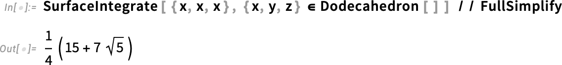
Functions like D and Integrate—as well as LineIntegrate and SurfaceIntegrate—are, in a sense, “classic calculus”, taught and used for more than three centuries. But in Version 14 we also support what we can think of as “emerging” calculus operations, like fractional differentiation:
\n
What are the primitives from which we can best build our conception of computation? That’s at some level the question I’ve been asking for more than four decades, and what’s determined the functions and structures at the core of the Wolfram Language.
\nAnd as the years go by, and we see more and more of what’s possible, we recognize and invent new primitives that will be useful. And, yes, the world—and the ways people interact with computers—change too, opening up new possibilities and bringing new understanding of things. Oh, and this year there are LLMs which can “get the intellectual sense of the world” and suggest new functions that can fit into the framework we’ve created with the Wolfram Language. (And, by the way, there’ve also been lots of great suggestions made by the audiences of our design review livestreams.)
\nOne new construct added in Version 13.1—and that I personally have found very useful—is Threaded. When a function is listable—as Plus is—the top levels of lists get combined:
\nBut sometimes you want one list to be “threaded into” the other at the lowest level, not the highest. And now there’s a way to specify that, using Threaded:
\nIn a sense, Threaded is part of a new wave of symbolic constructs that have “ambient effects” on lists. One very simple example (introduced in 2015) is Nothing:
\nAnother, introduced in 2020, is Splice:
\nAn old chestnut of Wolfram Language design concerns the way infinite evaluation loops are handled. And in Version 13.2 we introduced the symbolic construct TerminatedEvaluation to provide better definition of how out-of-control evaluations have been terminated:
\n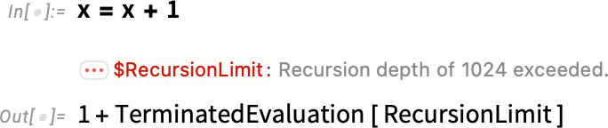
In a curious connection, in the computational representation of physics in our recent Physics Project, the direct analog of nonterminating evaluations are what make possible the seemingly unending universe in which we live.
\nBut what is actually going on “inside an evaluation”, terminating or not? I’ve always wanted a good representation of this. And in fact back in Version 2.0 we introduced Trace for this purpose:
\nBut just how much detail of what the evaluator does should one show? Back in Version 2.0 we introduced the option TraceOriginal that traces every path followed by the evaluator:
\nBut often this is way too much. And in Version 14.0 we’ve introduced the new setting TraceOriginal→Automatic, which doesn’t include in its output evaluations that don’t do anything:
\nThis may seem pedantic, but when one has an expression of any substantial size, it’s a crucial piece of pruning. So, for example, here’s a graphical representation of a simple arithmetic evaluation, with TraceOriginal→True:
\n
And here’s the corresponding “pruned” version, with TraceOriginal→Automatic:
\n
(And, yes, the structures of these graphs are closely related to things like the causal graphs we construct in our Physics Project.)
\nIn the effort to add computational primitives to the Wolfram Language, two new entrants in Version 14.0 are Comap and ComapApply. The function Map takes a function f and “maps it” over a list:
\nComap does the “mathematically co-” version of this, taking a list of functions and “comapping” them onto a single argument:
\nWhy is this useful? As an example, one might want to apply three different statistical functions to a single list. And now it’s easy to do that, using Comap:
\n
By the way, as with Map, there’s also an operator form for Comap:
\n
Comap works well when the functions it’s dealing with take just one argument. If one has functions that take multiple arguments, ComapApply is what one typically wants:
\nTalking of “co-like” functions, a new function added in Version 13.2 is PositionSmallest. Min gives the smallest element in a list; PositionSmallest instead says where the smallest elements are:
\nOne of the important objectives in the Wolfram Language is to have as much as possible “just work”. When we released Version 1.0 strings could be assumed just to contain ordinary ASCII characters, or perhaps to have an external character encoding defined. And, yes, it could be messy not to know “within the string itself” what characters were supposed to be there. And by the time of Version 3.0 in 1996 we’d become contributors to, and early adopters of, Unicode, which provided a standard encoding for “16-bits’-worth” of characters. And for many years this served us well. But in time—and particularly with the growth of emoji—16 bits wasn’t enough to encode all the characters people wanted to use. So a few years ago we began rolling out support for 32-bit Unicode, and in Version 13.1 we integrated it into notebooks—in effect making strings something much richer than before:
\nAnd, yes, you can use Unicode everywhere now:
\n
Back when Version 1.0 was released, a megabyte was a lot of memory. But 35 years later we routinely deal with gigabytes. And one of the things that makes practical is computation with video. We first introduced Video experimentally in Version 12.1 in 2020. And over the past three years we’ve been systematically broadening and strengthening our ability to deal with video in Wolfram Language. Probably the single most important advance is that things around video now—as much as possible—“just work”, without “creaking” under the strain of handling such large amounts of data.
\nWe can directly capture video into notebooks, and we can robustly play video anywhere within a notebook. We’ve also added options for where to store the video so that it’s conveniently accessible to you and anyone else you want to give access to it.
\nThere’s lots of complexity in the encoding of video—and we now robustly and transparently support more than 500 codecs. We also do lots of convenient things automatically, like rotating portrait-mode videos—and being able to apply image processing operations like ImageCrop across whole videos. In every version, we’ve been further optimizing the speed of some video operation or another.
\nBut a particularly big focus has been on video generators: programmatic ways to produce videos and animations. One basic example is AnimationVideo, which produces the same kind of output as Animate, but as a Video object that can either be displayed directly in a notebook, or exported in MP4 or some other format:
\n
AnimationVideo is based on computing each frame in a video by evaluating an expression. Another class of video generators take an existing visual construct, and simply “tour” it. TourVideo “tours” images, graphics and geo graphics; Tour3DVideo (new in Version 14.0) tours 3D geometry:
\n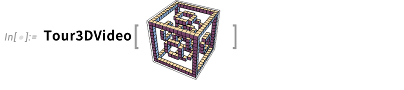
A very powerful capability in Wolfram Language is being able to apply arbitrary functions to videos. One example of how this can be done is VideoFrameMap, which maps a function across frames of a video, and which was made efficient in Version 13.2:
\n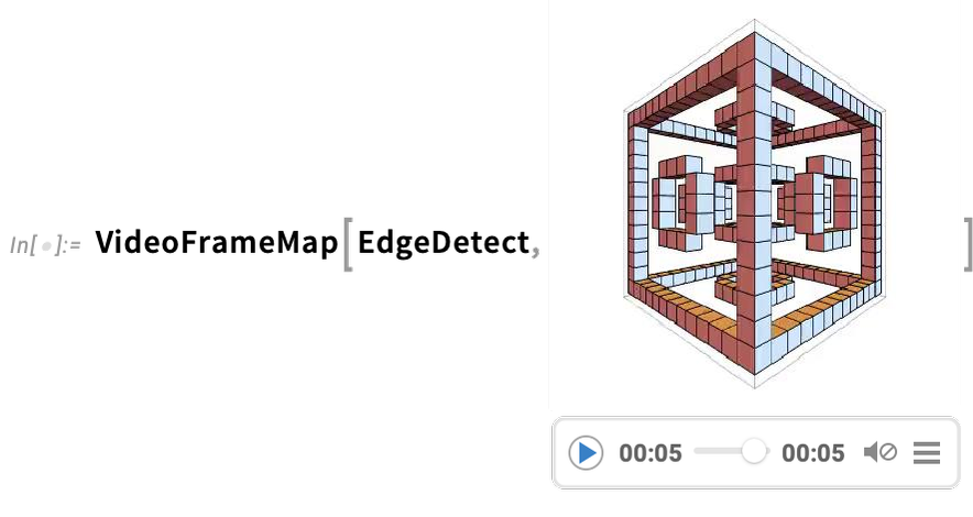
And although Wolfram Language isn’t intended as an interactive video editing system, we’ve made sure that it’s possible to do streamlined programmatic video editing in the language, and for example in Version 14.0 we’ve added things like transition effects in VideoJoin and timed overlays in OverlayVideo.
\nWith every new version of Wolfram Language we add new capabilities to extend yet further the domain of the language. But we also put a lot of effort into something less immediately visible: making existing capabilities faster, stronger and sleeker.
\nAnd in Version 14 two areas where we can see some examples of all these are dates and quantities. We introduced the notion of symbolic dates (DateObject, etc.) nearly a decade ago. And over the years since then we’ve built many things on this structure. And in the process of doing this it’s become clear that there are certain flows and paths that are particularly common and convenient. At the beginning what mattered most was just to make sure that the relevant functionality existed. But over time we’ve been able to see what should be streamlined and optimized, and we’ve steadily been doing that.
\nIn addition, as we’ve worked towards new and different applications, we’ve seen “corners” that need to be filled in. So, for example, astronomy is an area we’ve significantly developed in Version 14, and supporting astronomy has required adding several new “high-precision” time capabilities, such as the TimeSystem option, as well as new astronomy-oriented calendar systems. Another example concerns date arithmetic. What should happen if you want to add a month to January 30? Where should you land? Different kinds of business applications and contracts make different assumptions—and so we added a Method option to functions like DatePlus to handle this. Meanwhile, having realized that date arithmetic is involved in the “inner loop” of certain computations, we optimized it—achieving a more than 100x speedup in Version 14.0.
\nWolfram|Alpha has been able to deal with units ever since it was first launched in 2009—now more than 10,000 of them. And in 2012 we introduced Quantity to represent quantities with units in the Wolfram Language. And over the past decade we’ve been steadily smoothing out a whole series of complicated gotchas and issues with units. For example, what does ![]() .
.
At first our priority with Quantity was to get it working as broadly as possible, and to integrate it as widely as possible into computations, visualizations, etc. across the system. But as its capabilities have expanded, so have its uses, repeatedly driving the need to optimize its operation for particular common cases. And indeed between Version 13 and Version 14 we’ve dramatically sped up many things related to Quantity, often by factors of 1000 or more.
\nTalking of speedups, another example—made possible by new algorithms operating on multithreaded CPUs—concerns polynomials. We’ve worked with polynomials in Wolfram Language since Version 1, but in Version 13.2 there was a dramatic speedup of up to 1000x on operations like polynomial factoring.
\nIn addition, a new algorithm in Version 14.0 dramatically speeds up numerical solutions to polynomial and transcendental equations—and, together with the new MaxRoots options, allows us, for example, to pick off a few roots from a degree-one-million polynomial
\n
or to find roots of a transcendental equation that we could not even attempt before without pre-specifying bounds on their values:
\n
Another “old” piece of functionality with recent enhancement concerns mathematical functions. Ever since Version 1.0 we’ve set up mathematical functions so that they can be computed to arbitrary precision:
\nBut in recent versions we’ve wanted to be “more precise about precision”, and to be able to rigorously compute just what range of outputs are possible given the range of values provided as input:
\nBut every function for which we do this effectively requires a new theorem, and we’ve been steadily increasing the number of functions covered—now more than 130—so that this “just works” when you need to use it in a computation.
\nTrees are useful. We first introduced them as basic objects in the Wolfram Language only in Version 12.3. But now that they’re there, we’re discovering more and more places they can be used. And to support that, we’ve been adding more and more capabilities to them.
\nOne area that’s advanced significantly since Version 13 is the rendering of trees. We tightened up the general graphic design, but, more importantly, we introduced many new options for how rendering should be done.
\nFor example, here’s a random tree where we’ve specified that for all nodes only 3 children should be explicitly displayed: the others are elided away:
\n
Here we’re adding several options to define the rendering of the tree:
\n
By default, the branches in trees are labeled with integers, just like parts in an expression. But in Version 13.1 we added support for named branches defined by associations:
\n
Our original conception of trees was very centered around having elements one would explicitly address, and that could have “payloads” attached. But what became clear is that there were applications where all that mattered was the structure of the tree, not anything about its elements. So we added UnlabeledTree to create “pure trees”:
\n
Trees are useful because many kinds of structures are basically trees. And since Version 13 we’ve added capabilities for converting trees to and from various kinds of structures. For example, here’s a simple Dataset object:
\n
You can use ExpressionTree to convert this to a tree:
\n
And TreeExpression to convert it back:
\n
We’ve also added capabilities for converting to and from JSON and XML, as well as for representing file directory structures as trees:
\n
In Version 1.0 we had integers, rational numbers and real numbers. In Version 3.0 we added algebraic numbers (represented implicitly by Root)—and a dozen years later we added algebraic number fields and transcendental roots. For Version 14 we’ve now added another (long-awaited) “number-related” construct: finite fields.
\nHere’s our symbolic representation of the field of integers modulo 7:
\n
And now here’s a specific element of that field
\n
which we can immediately compute with:
\n
But what’s really important about what we’ve done with finite fields is that we’ve fully integrated them into other functions in the system. So, for example, we can factor a polynomial whose coefficients are in a finite field:
\n
We can also do things like find solutions to equations over finite fields. So here, for example, is a point on a Fermat curve over the finite field GF(173):
\n
And here is a power of a matrix with elements over the same finite field:
\n
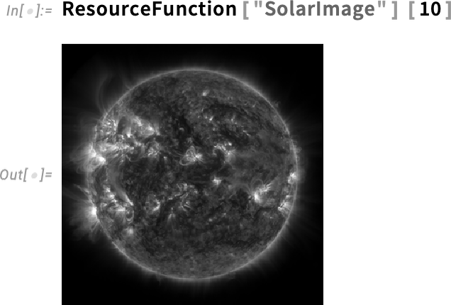
A major new capability added since Version 13 is astro computation. It begins with being able to compute to high precision the positions of things like planets. Even knowing what one means by “position” is complicated, though—with lots of different coordinate systems to deal with. By default AstroPosition gives the position in the sky at the current time from your Here location:
\n
But one can instead ask about a different coordinate system, like global galactic coordinates:
\n
And now here’s a plot of the distance between Saturn and Jupiter over a 50-year period:
\n
In direct analogy to GeoGraphics, we’ve added AstroGraphics, here showing a patch of sky around the current position of Saturn:
\n
And this now shows the sequence of positions for Saturn over the course of a couple of years—yes, including retrograde motion:
\n
There are many styling options for AstroGraphics. Here we’re adding a background of the “galactic sky”:
\n
And here we’re including renderings for constellations (and, yes, we had an artist draw them):
\n
Something specifically new in Version 14.0 has to do with extended handling of solar eclipses. We always try to deliver new functionality as fast as we can. But in this case there was a very specific deadline: the total solar eclipse visible from the US on April 8, 2024. We’ve had the ability to do global computations about solar eclipses for some time (actually since soon before the 2017 eclipse). But now we can also do detailed local computations right in the Wolfram Language.
\nSo, for example, here’s a somewhat detailed overall map of the April 8, 2024, eclipse:
\n
Now here’s a plot of the magnitude of the eclipse over a few hours, complete with a little “rampart” associated with the period of totality:
\n
And here’s a map of the region of totality every minute just after the moment of maximum eclipse:
\n
We first introduced computable data on biological organisms back when Wolfram|Alpha was released in 2009. But in Version 14—following several years of work—we’ve dramatically broadened and deepened the computable data we have about biological organisms.
\nSo for example here’s how we can figure out what species have cheetahs as predators:
\n
And here are pictures of these:
\n
Here’s a map of countries where cheetahs have been seen (in the wild):
\n
We now have data—curated from a great many sources—on more than a million species of animals, as well as most of the plants, fungi, bacteria, viruses and archaea that have been described. And for animals, for example, we have nearly 200 properties that are extensively filled in. Some are taxonomic properties:
\n
Some are physical properties:
\n

Some are genetic properties:
\n
Some are ecological properties (yes, the cheetah is not the apex predator):
\n
It’s useful to be able to get properties of individual species, but the real power of our curated computable data shows up when one does larger-scale analyses. Like here’s a plot of the lengths of genomes for organisms with the longest ones across our collection of organisms:
\n
Or here’s a histogram of the genome lengths for organisms in the human gut microbiome:
\n
And here’s a scatterplot of the lifespans of birds against their weights:
\n
Following the idea that cheetahs aren’t apex predators, this is a graph of what’s “above” them in the food chain:
\n
We began the process of introducing chemical computation into the Wolfram Language in Version 12.0, and by Version 13 we had good coverage of atoms, molecules, bonds and functional groups. Now in Version 14 we’ve added coverage of chemical formulas, amounts of chemicals—and chemical reactions.
\nHere’s a chemical formula, that basically just gives a “count of atoms”:
\n
Now here are specific molecules with that formula:
\n
Let’s pick one of these molecules:
\n
Now in Version 14 we have a way to represent a certain quantity of molecules of a given type—here 1 gram of methylcyclopentane:
\n
ChemicalConvert can convert to a different specification of quantity, here moles:
\n
And here a count of molecules:
\n
But now the bigger story is that in Version 14 we can represent not just individual types of molecules, and quantities of molecules, but also chemical reactions. Here we give a “sloppy” unbalanced representation of a reaction, and ReactionBalance gives us the balanced version:
\n
And now we can extract the formulas for the reactants:
\n
We can also give a chemical reaction in terms of molecules:
\n
But with our symbolic representation of molecules and reactions, there’s now a big thing we can do: represent classes of reactions as “pattern reactions”, and work with them using the same kinds of concepts as we use in working with patterns for general expressions. So, for example, here’s a symbolic representation of the hydrohalogenation reaction:
\n
Now we can apply this pattern reaction to particular molecules:
\n
Here’s a more elaborate example, in this case entered using a SMARTS string:
\n
Here we’re applying the reaction just once:
\n
And now we’re doing it repeatedly
\n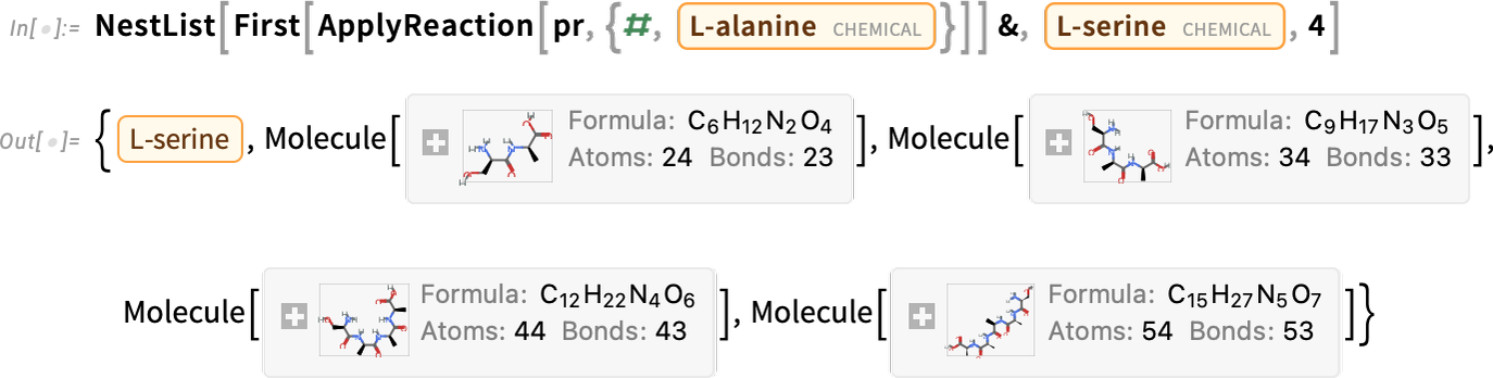
in this case generating longer and longer molecules (which in this case happen to be polypeptides):
\n
Every minute of every day, new data is being added to the Wolfram Knowledgebase. Much of it is coming automatically from real-time feeds. But we also have a very large-scale ongoing curation effort with humans in the loop. We’ve built sophisticated (Wolfram Language) automation for our data curation pipeline over the years—and this year we’ve been able to increase efficiency in some areas by using LLM technology. But it’s hard to do curation right, and our long-term experience is that to do so ultimately requires human experts being in the loop, which we have.
\nSo what’s new since Version 13.0? 291,842 new notable current and historical people; 264,467 music works; 118,538 music albums; 104,024 named stars; and so on. Sometimes the addition of an entity is driven by the new availability of reliable data; often it’s driven by the need to use that entity in some other piece of functionality (e.g. stars to render in AstroGraphics). But more than just adding entities there’s the issue of filling in values of properties of existing entities. And here again we’re always making progress, sometimes integrating newly available large-scale secondary data sources, and sometimes doing direct curation ourselves from primary sources.
\nA recent example where we needed to do direct curation was in data on alcoholic beverages. We have very extensive data on hundreds of thousands of types of foods and drinks. But none of our large-scale sources included data on alcoholic beverages. So that’s an area where we need to go to primary sources (in this case typically the original producers of products) and curate everything for ourselves.
\nSo, for example, we can now ask for something like the distribution of flavors of different varieties of vodka (actually, personally, not being a consumer of such things, I had no idea vodka even had flavors…):
\n
But beyond filling out entities and properties of existing types, we’ve also steadily been adding new entity types. One recent example is geological formations, 13,706 of them:
\n
So now, for example, we can specify where T. rex have been found
\n
and we can show those regions on a map:
\n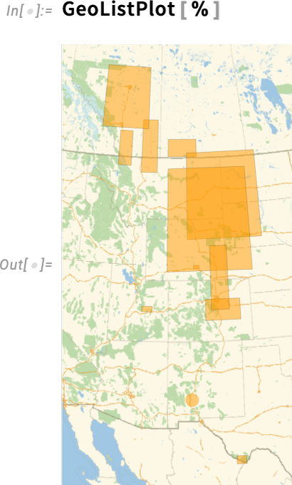
PDEs are hard. It’s hard to solve them. And it’s hard to even specify what exactly you want to solve. But we’ve been on a multi-decade mission to “consumerize” PDEs and make them easier to work with. Many things go into this. You need to be able to easily specify elaborate geometries. You need to be able to easily define mathematically complicated boundary conditions. You need to have a streamlined way to set up the complicated equations that come out of underlying physics. Then you have to—as automatically as possible—do the sophisticated numerical analysis to efficiently solve the equations. But that’s not all. You also often need to visualize your solution, compute other things from it, or run optimizations of parameters over it.
\nIt’s a deep use of what we’ve built with Wolfram Language—touching many parts of the system. And the result is something unique: a truly streamlined and integrated way to handle PDEs. One’s not dealing with some (usually very expensive) “just for PDEs” package; what we now have is a “consumerized” way to handle PDEs whenever they’re needed—for engineering, science, or whatever. And, yes, being able to connect machine learning, or image computation, or curated data, or data science, or real-time sensor feeds, or parallel computing, or, for that matter, Wolfram Notebooks, to PDEs just makes them so much more valuable.
\nWe’ve had “basic, raw NDSolve” since 1991. But what’s taken decades to build is all the structure around that to let one conveniently set up—and efficiently solve—real-world PDEs, and connect them into everything else. It’s taken developing a whole tower of underlying algorithmic capabilities such as our more-flexible-and-integrated-than-ever-before industrial-strength computational geometry and finite element methods. But beyond that it’s taken creating a language for specifying real-world PDEs. And here the symbolic nature of the Wolfram Language—and our whole design framework—has made possible something very unique, that has allowed us to dramatically simplify and consumerize the use of PDEs.
\nIt’s all about providing symbolic “construction kits” for PDEs and their boundary conditions. We started this about five years ago, progressively covering more and more application areas. In Version 14 we’ve particularly focused on solid mechanics, fluid mechanics, electromagnetics and (one-particle) quantum mechanics.
\nHere’s an example from solid mechanics. First, we define the variables we’re dealing with (displacement and underlying coordinates):
\nNext, we specify the parameters we want to use to describe the solid material we’re going to work with:
\nNow we can actually set up our PDE—using symbolic PDE specifications like SolidMechanicsPDEComponent—here for the deformation of a solid object pulled on one side:
\n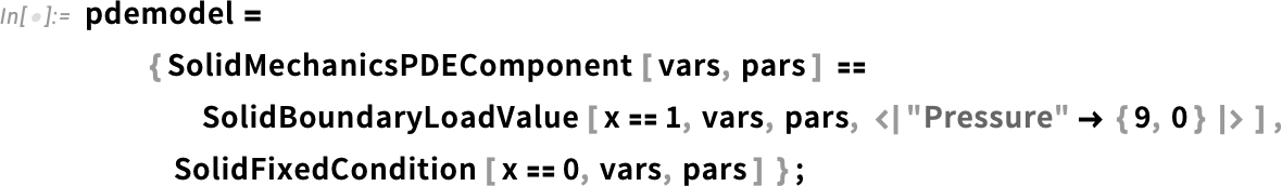
And, yes, “underneath”, these simple symbolic specifications turn into a complicated “raw” PDE:
\n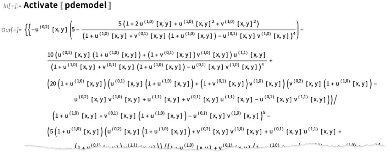
Now we are ready to actually solve our PDE in a particular region, i.e. for an object with a particular shape:
\n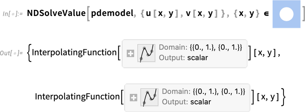
And now we can visualize the result, which shows how our object stretches when it’s pulled on:
\n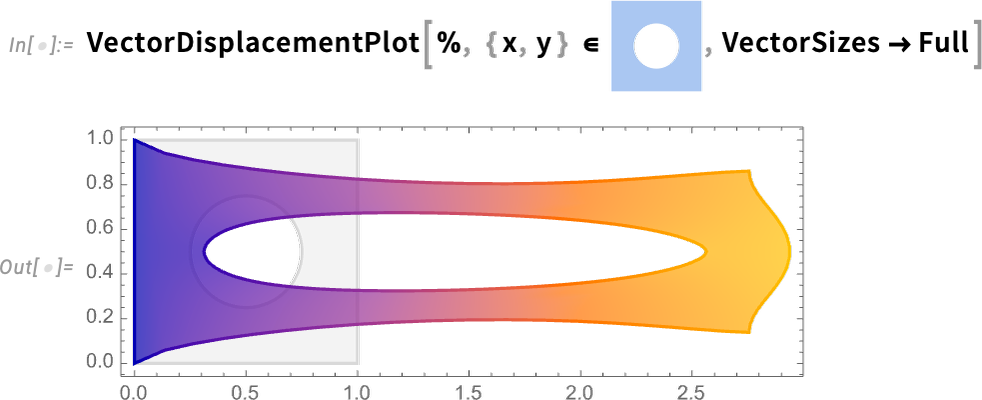
The way we’ve set things up, the material for our object is an idealization of something like rubber. But in the Wolfram Language we now have ways to specify all sorts of detailed properties of materials. So, for example, we can add reinforcement as a unit vector in a particular direction (say in practice with fibers) to our material:
\nThen we can rerun what we did before
\n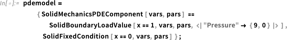
but now we get a slightly different result:
\n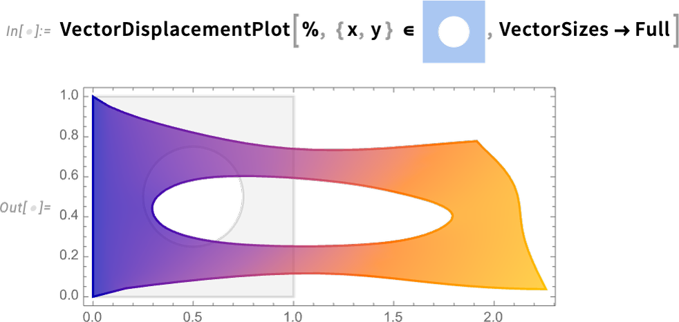
Another major PDE domain that’s new in Version 14.0 is fluid flow. Let’s do a 2D example. Our variables are 2D velocity and pressure:
\nNow we can set up our fluid system in a particular region, with no-slip conditions on all walls except at the top where we assume fluid is flowing from left to right. The only parameter needed is the Reynolds number. And instead of just solving our PDEs for a single Reynolds number, let’s create a parametric solver that can take any specified Reynolds number:
\n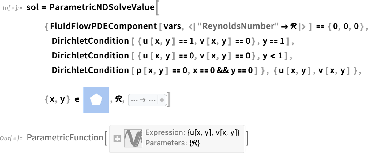
Now here’s the result for Reynolds number 100:
\n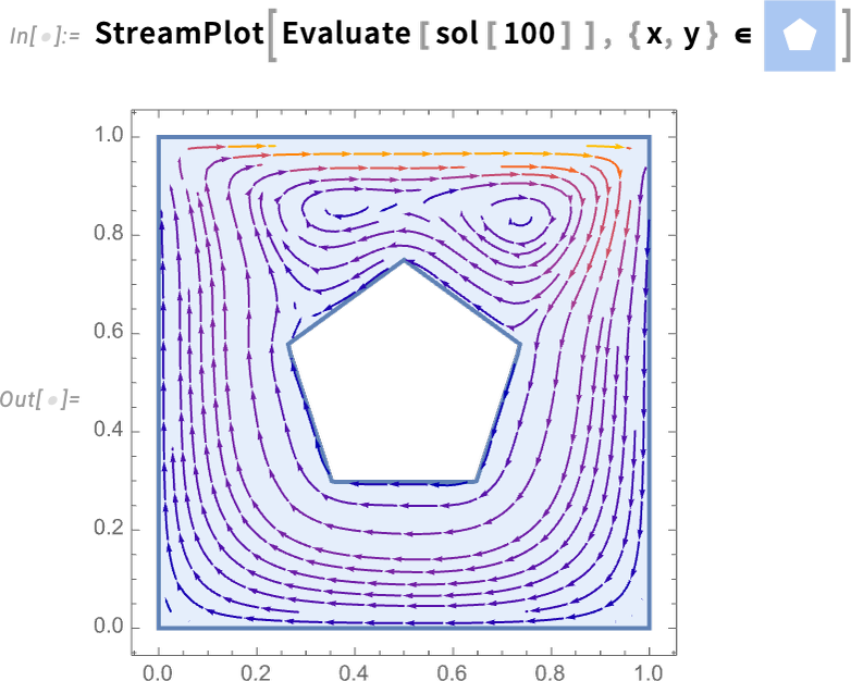
But with the way we’ve set things up, we can as well generate a whole video as a function of Reynolds number (and, yes, the Parallelize speeds things up by generating different frames in parallel):
\n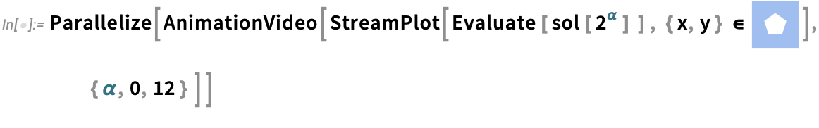
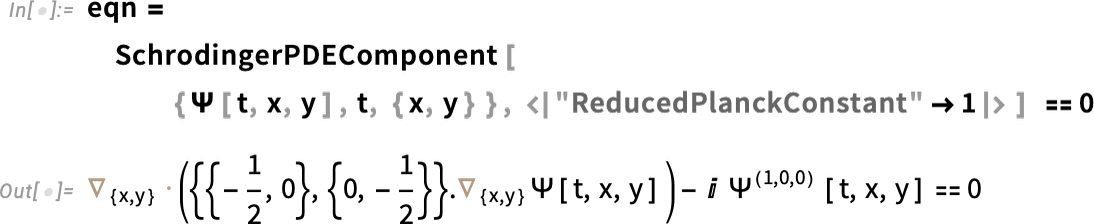
Much of our work in PDEs involves catering to the complexities of real-world engineering situations. But in Version 14.0 we’re also adding features to support “pure physics”, and in particular to support quantum mechanics done with the Schrödinger equation. So here, for example, is the 2D 1-particle Schrödinger equation (with ![]() ):
):
Here’s the region we’re going to be solving over—showing explicit discretization:
\n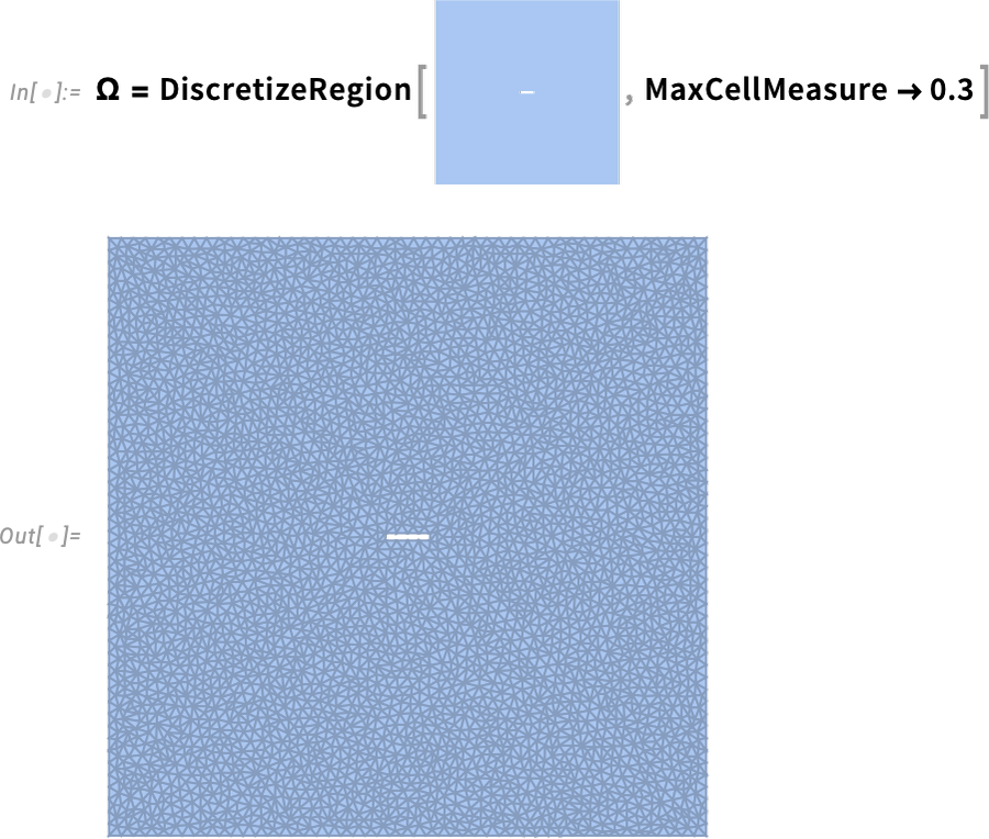
Now we can solve the equation, adding in some boundary conditions:
\n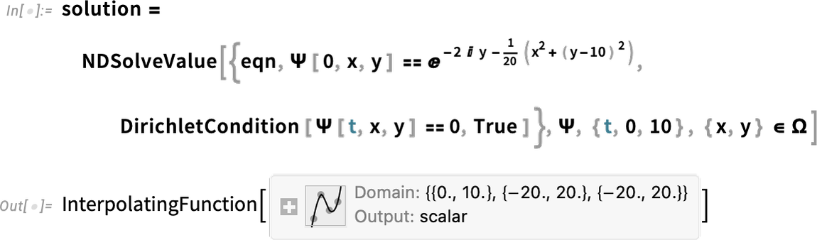
And now we get to visualize a Gaussian wave packet scattering around a barrier:
\n
Systems engineering is a big field, but it’s one where the structure and capabilities of the Wolfram Language provide unique advantages—that over the past decade have allowed us to build out rather complete industrial-strength support for modeling, analysis and control design for a wide range of types of systems. It’s all an integrated part of the Wolfram Language, accessible through the computational and interface structure of the language. But it’s also integrated with our separate Wolfram System Modeler product, that provides a GUI-based workflow for system modeling and exploration.
\nShared with System Modeler are large collections of domain-specific modeling libraries. And, for example, since Version 13, we’ve added libraries in areas such as battery engineering, hydraulic engineering and aircraft engineering—as well as educational libraries for mechanical engineering, thermal engineering, digital electronics, and biology. (We’ve also added libraries for areas such as business and public policy simulation.)
\n
A typical workflow for systems engineering begins with the setting up of a model. The model can be built from scratch, or assembled from components in model libraries—either visually in Wolfram System Modeler, or programmatically in the Wolfram Language. For example, here’s a model of an electric motor that’s turning a load through a flexible shaft:
\n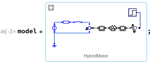
Once one’s got a model, one can then simulate it. Here’s an example where we’ve set one parameter of our model (the moment of inertia of the load), and we’re computing the values of two others as a function of time:
\n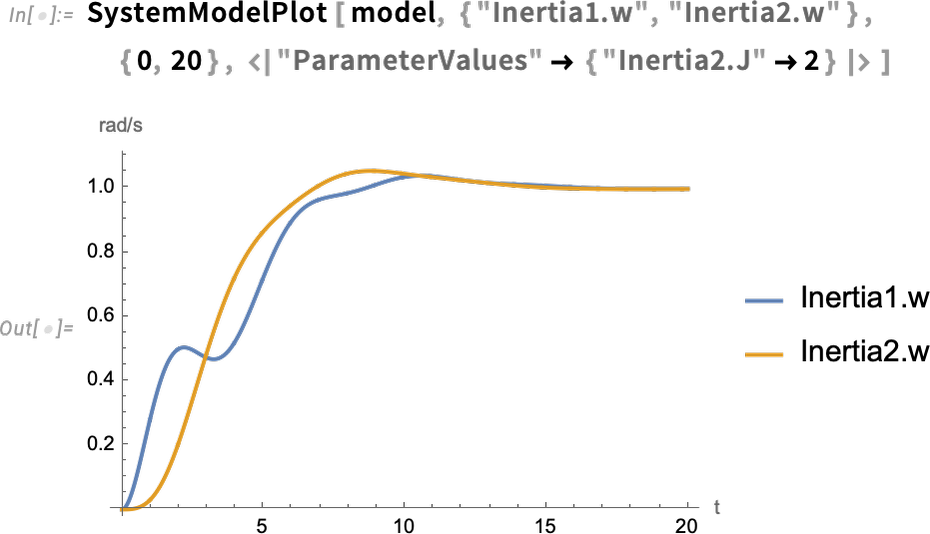
A new capability in Version 14.0 is being able to see the effect of uncertainty in parameters (or initial values, etc.) on the behavior of a system. So here, as an example, we’re saying the value of the parameter is not definite, but is instead distributed according to a normal distribution—then we’re seeing the distribution of output results:
\n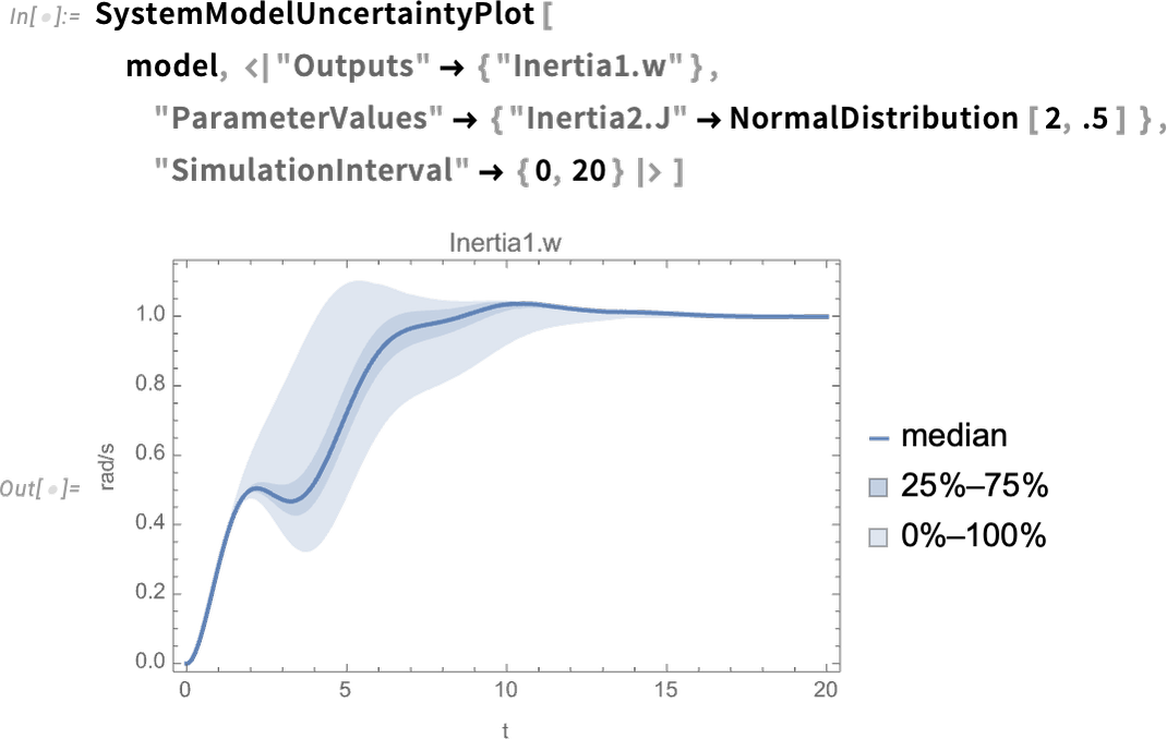
The motor with flexible shaft that we’re looking at can be thought of as a “multidomain system”, combining electrical and mechanical components. But the Wolfram Language (and Wolfram System Modeler) can also handle “mixed systems”, combining analog and digital (i.e. continuous and discrete) components. Here’s a fairly sophisticated example from the world of control systems: a helicopter model connected in a closed loop to a digital control system:
\n
This whole model system can be represented symbolically just by:
\nAnd now we compute the input-output response of the model:
\n
Here’s specifically the output response:
\n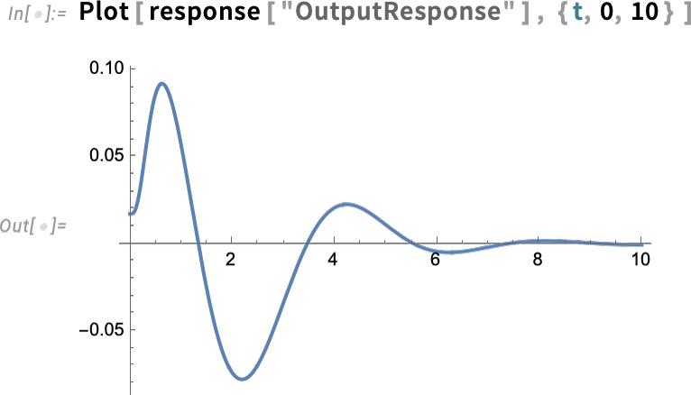
But now we can “drill in” and see specific subsystem responses, here of the zero-order hold device (labeled ZOH above)—complete with its little digital steps:
\n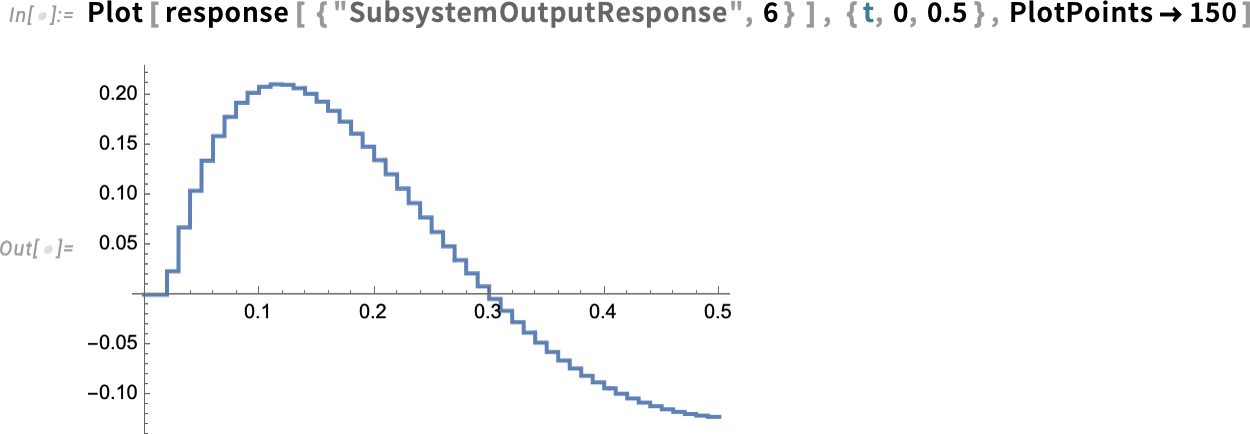
But what if we want to design the control systems ourselves? Well, in Version 14 we can now apply all our Wolfram Language control systems design functionality to arbitrary system models. Here’s an example of a simple model, in this case in chemical engineering (a continuously stirred tank):
\n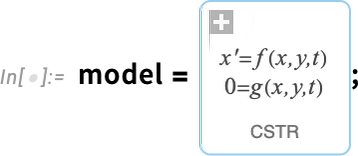
Now we can take this model and design an LQG controller for it—then assemble a whole closed-loop system for it:
\n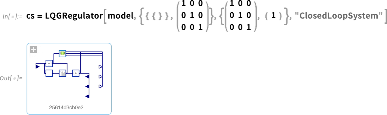
Now we can simulate the closed-loop system—and see that the controller succeeds in bringing the final value to 0:
\n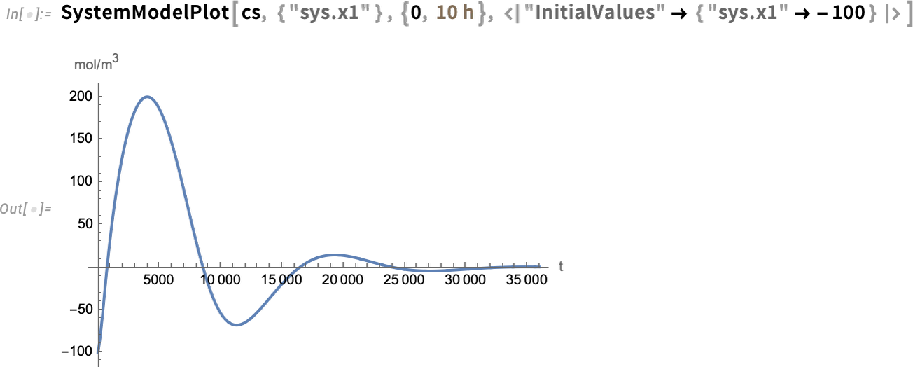
Graphics have always been an important part of the story of the Wolfram Language, and for more than three decades we’ve been progressively enhancing and updating their appearance and functionality—sometimes with help from advances in hardware (e.g. GPU) capabilities.
\nSince Version 13 we’ve added a variety of “decorative” (or “annotative”) effects in 2D graphics. One example (useful for putting captions on things) is Haloing:
\n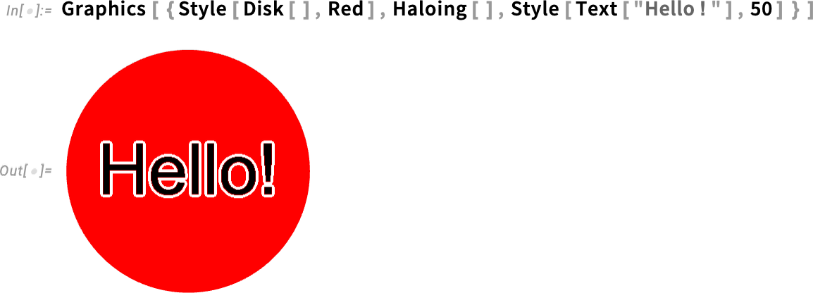
Another example is DropShadowing:
\n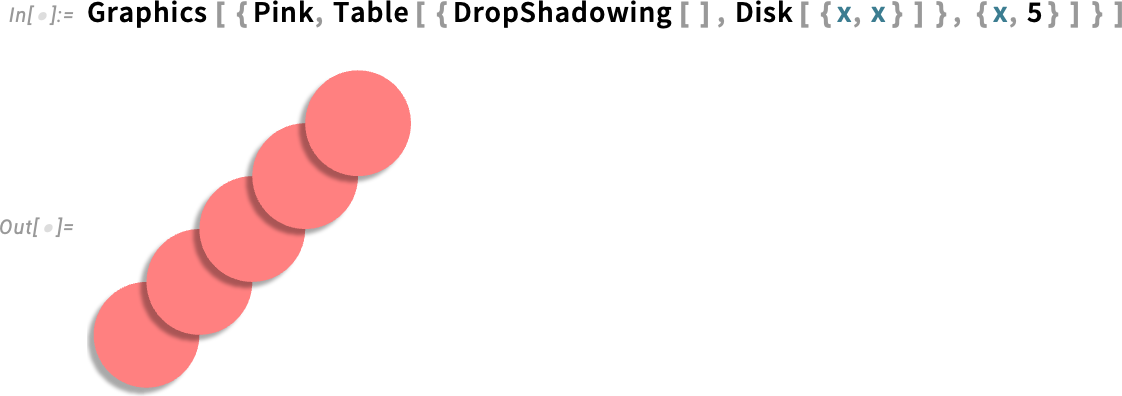
All of these are specified symbolically, and can be used throughout the system (e.g. in hover effects, etc). And, yes, there are many detailed parameters you can set:
\n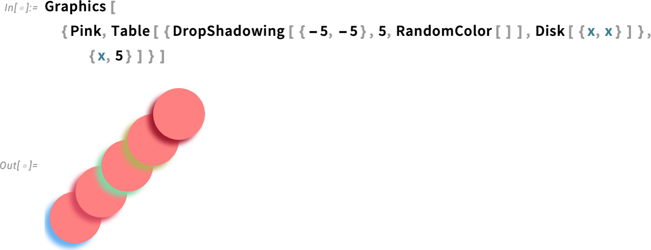
A significant new capability in Version 14.0 is convenient texture mapping. We’ve had low-level polygon-by-polygon textures for a decade and a half. But now in Version 14.0 we’ve made it straightforward to map textures onto whole surfaces. Here’s an example wrapping a texture onto a sphere:
\n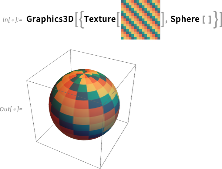
And here’s wrapping the same texture onto a more complicated surface:
\n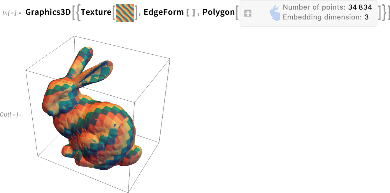
A significant subtlety is that there are many ways to map what amount to “texture coordinate patches” onto surfaces. The documentation illustrates new, named cases:
\n
And now here’s what happens with stereographic projection onto a sphere:
\n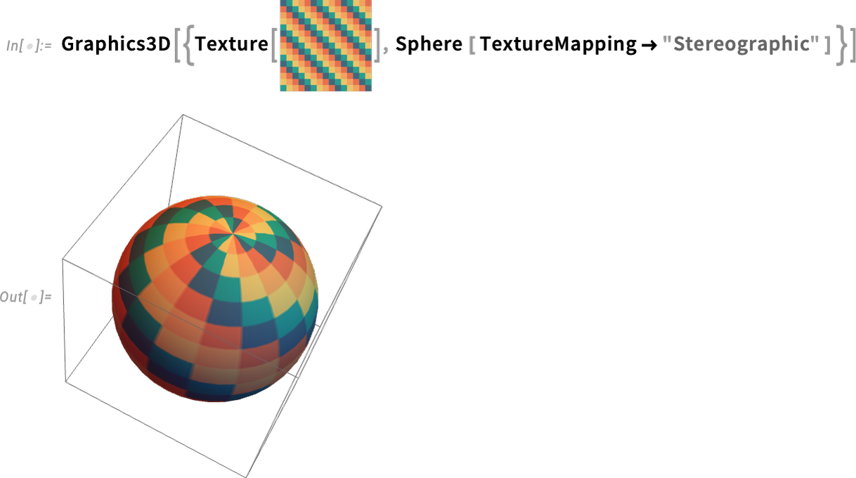
Here’s an example of “surface texture” for the planet Venus
\n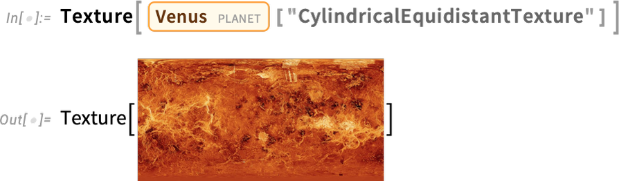
and here it’s been mapped onto a sphere, which can be rotated:
\n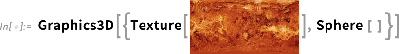
Here’s a “flowerified” bunny:
\n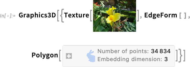
Things like texture mapping help make graphics visually compelling. Since Version 13 we’ve also added a variety of “live visualization” capabilities that automatically “bring visualizations to life”. For example, any plot now by default has a “coordinate mouseover”:
\n
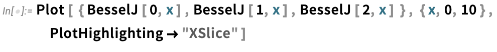
As usual, there’s lots of ways to control such “highlighting” effects:
\n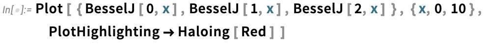
One might say it’s been two thousand years in the making. But four years ago (Version 12) we began to introduce a computable version of Euclid-style synthetic geometry.
\nThe idea is to specify geometric scenes symbolically by giving a collection of (potentially implicit) constraints:
\n
We can then generate a random instance of geometry consistent with the constraints—and in Version 14 we’ve considerably enhanced our ability to make sure that geometry will be “typical” and non-degenerate:
\n
But now a new feature of Version 14 is that we can find values of geometric quantities that are determined by the constraints:
\n
Here’s a slightly more complicated case:
\n
And here we’re now solving for the areas of two triangles in the figure:
\n
We’ve always been able to give explicit styles for particular elements of a scene:
\n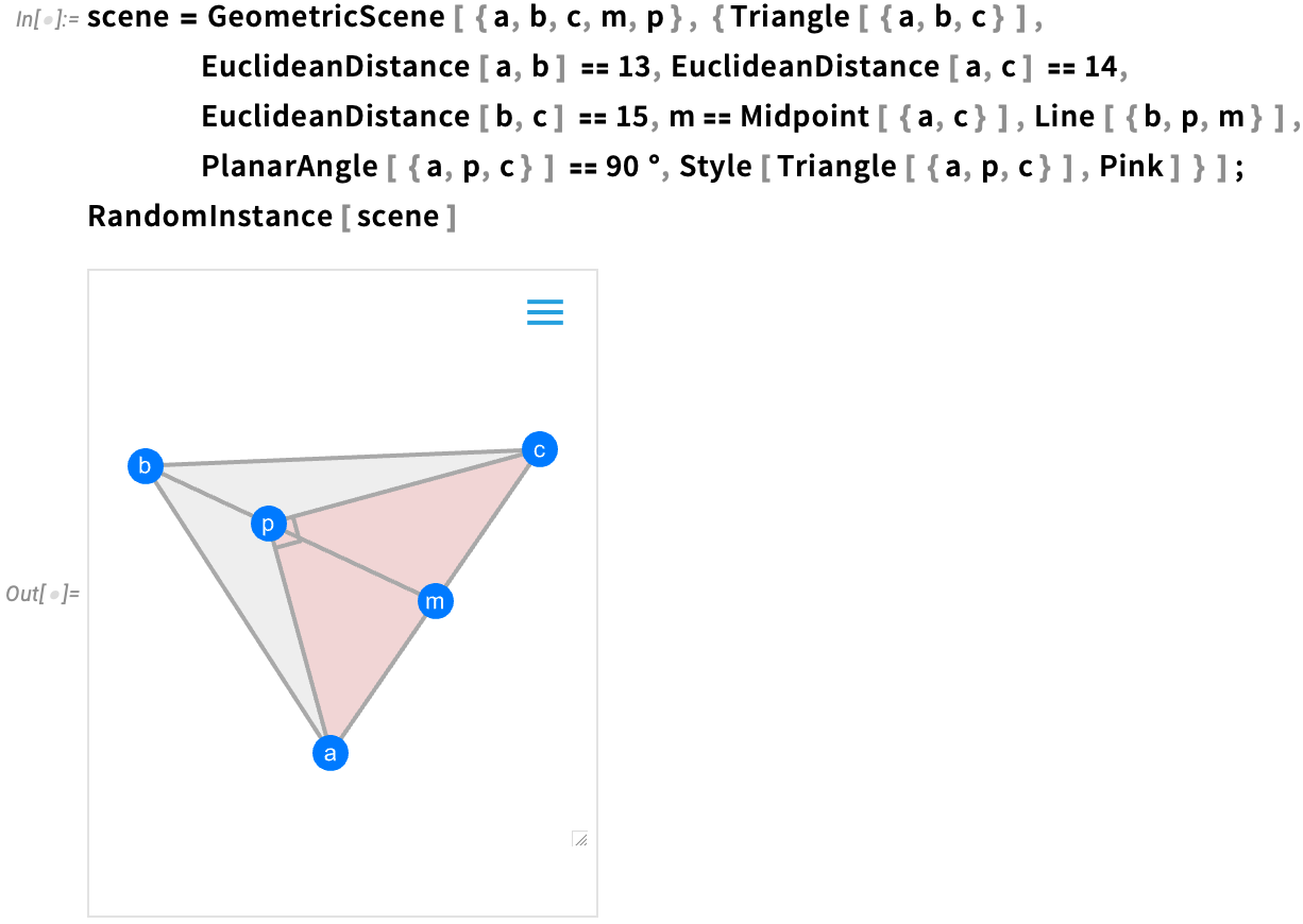
Now one of the new features in Version 14 is being able to give general “geometric styling rules”, here just assigning random colors to each element:
\n
Our goal with Wolfram Language is to make it as easy as possible to express oneself computationally. And a big part of achieving that is the coherent design of the language itself. But there’s another part as well, which is being able to actually enter Wolfram Language input one wants—say in a notebook—as easily as possible. And with every new version we make enhancements to this.
\nOne area that’s been in continuous development is interactive syntax highlighting. We first added syntax highlighting nearly two decades ago—and over time we’ve progressively made it more and more sophisticated, responding both as you type, and as code gets executed. Some highlighting has always had obvious meaning. But particularly highlighting that is dynamic and based on cursor position has sometimes been harder to interpret. And in Version 14—leveraging the brighter color palettes that have become the norm in recent years—we’ve tuned our dynamic highlighting so it’s easier to quickly tell “where you are” within the structure of an expression:
\n
On the subject of “knowing what one has”, another enhancement—added in Version 13.2—is differentiated frame coloring for different kinds of visual objects in notebooks. Is that thing one has a graphic? Or an image? Or a graph? Now one can tell from the color of frame when one selects it:
\n
An important aspect of the Wolfram Language is that the names of built-in functions are spelled out enough that it’s easy to tell what they do. But often the names are therefore necessarily quite long, and so it’s important to be able to autocomplete them when one’s typing. In 13.3 we added the notion of “fuzzy autocompletion” that not only “completes to the end” a name one’s typing, but also can fill in intermediate letters, change capitalization, etc. Thus, for example, just typing lll brings up an autocompletion menu that begins with ListLogLogPlot:
\n 
A major user interface update that first appeared in Version 13.1—and has been enhanced in subsequent versions—is a default toolbar for every notebook:
\n![]()
The toolbar provides immediate access to evaluation controls, cell formatting and various kinds of input (like inline cells, ![]() , hyperlinks, drawing canvas, etc.)—as well as to things like
, hyperlinks, drawing canvas, etc.)—as well as to things like ![]() cloud publishing,
cloud publishing, ![]() documentation search and
documentation search and ![]() “chat” (i.e. LLM) settings.
“chat” (i.e. LLM) settings.
Much of the time, it’s useful to have the toolbar displayed in any notebook you’re working with. But on the left-hand side there’s a little tiny ![]() that lets you minimize the toolbar:
that lets you minimize the toolbar:

In 14.0 there’s a Preferences setting that makes the toolbar come up minimized in any new notebook you create—and this in effect gives you the best of both worlds: you have immediate access to the toolbar, but your notebooks don’t have anything “extra” that might distract from their content.
\nAnother thing that’s advanced since Version 13 is the handling of “summary” forms of output in notebooks. A basic example is what happens if you generate a very large result. By default only a summary of the result is actually displayed. But now there’s a bar at the bottom that gives various options for how to handle the actual output:
\n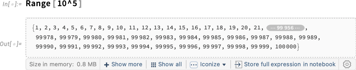
By default, the output is only stored in your current kernel session. But by pressing the Iconize button you get an iconized form that will appear directly in your notebook (or one that can be copied anywhere) and that “has the whole output inside”. There’s also a Store full expression in notebook button, which will “invisibly” store the output expression “behind” the summary display.
\nIf the expression is stored in the notebook, then it’ll be persistent across kernel sessions. Otherwise, well, you won’t be able to get to it in a different kernel session; the only thing you’ll have is the summary display:
\n
It’s a similar story for large “computational objects”. Like here’s a Nearest function with a million data points:
\n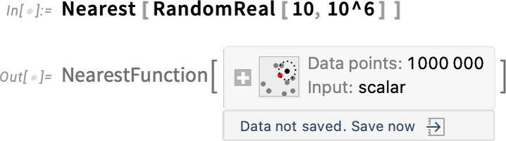
By default, the data is just something that exists in your current kernel session. But now there’s a menu that lets you save the data in various persistent locations:
\n
There are many ways to run the Wolfram Language. Even in Version 1.0 we had the notion of remote kernels: the notebook front end running on one machine (in those days essentially always a Mac, or a NeXT), and the kernel running on a different machine (in those days sometimes even connected by phone lines). But a decade ago came a major step forward: the Wolfram Cloud.
\nThere are really two distinct ways in which the cloud is used. The first is in delivering a notebook experience similar to our longtime desktop experience, but running purely in a browser. And the second is in delivering APIs and other programmatically accessed capabilities—notably, even at the beginning, a decade ago, through things like APIFunction.
\nThe Wolfram Cloud has been the target of intense development now for nearly 15 years. Alongside it have also come Wolfram Application Server and Wolfram Web Engine, which provide more streamlined support specifically for APIs (without things like user management, etc., but with things like clustering).
\nAll of these—but particularly the Wolfram Cloud—have become core technology capabilities for us, supporting many of our other activities. So, for example, the Wolfram Function Repository and Wolfram Paclet Repository are both based on the Wolfram Cloud (and in fact this is true of our whole resource system). And when we came to build the Wolfram plugin for ChatGPT earlier this year, using the Wolfram Cloud allowed us to have the plugin deployed within a matter of days.
\nSince Version 13 there have been quite a few very different applications of the Wolfram Cloud. One is for the function ARPublish, which takes 3D geometry and puts it in the Wolfram Cloud with appropriate metadata to allow phones to get augmented-reality versions from a QR code of a cloud URL:
\n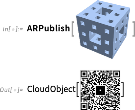

On the Cloud Notebook side, there’s been a steady increase in usage, notably of embedded Cloud Notebooks, which have for example become common on Wolfram Community, and are used all over the Wolfram Demonstrations Project. Our goal all along has been to make Cloud Notebooks be as easy to use as simple webpages, but to have the depth of capabilities that we’ve developed in notebooks over the past 35 years. We achieved this some years ago for fairly small notebooks, but in the past couple of years we’ve been going progressively further in handling even multi-hundred-megabyte notebooks. It’s a complicated story of caching, refreshing—and dodging the vicissitudes of web browsers. But at this point the vast majority of notebooks can be seamlessly deployed to the cloud, and will display as immediately as simple webpages.
\nIt’s been possible to call external code from Wolfram Language ever since Version 1.0. But in Version 14 there are important advances in the extent and ease with which external code can be integrated. The overall goal is to be able to use all the power and coherence of the Wolfram Language even when some part of a computation is done in external code. And in Version 14 we’ve done a lot to streamline and automate the process by which external code can be integrated into the language.
\nOnce something is integrated into the Wolfram Language it just becomes, for example, a function that can be used just like any other Wolfram Language function. But what’s underneath is necessarily quite different for different kinds of external code. There’s one setup for interpreted languages like Python. There’s another for C-like compiled languages and dynamic libraries. (And then there are others for external processes, APIs, and what amount to “importable code specifications”, say for neural networks.)
\nLet’s start with Python. We’ve had ExternalEvaluate for evaluating Python code since 2018. But when you actually come to use Python there are all these dependencies and libraries to deal with. And, yes, that’s one of the places where the incredible advantages of the Wolfram Language and its coherent design are painfully evident. But in Version 14.0 we now have a way to encapsulate all that Python complexity, so that we can deliver Python functionality within Wolfram Language, hiding all the messiness of Python dependencies, and even the versioning of Python itself.
\nAs an example, let’s say we want to make a Wolfram Language function Emojize that uses the Python function emojize within the emoji Python library. Here’s how we can do that:
\n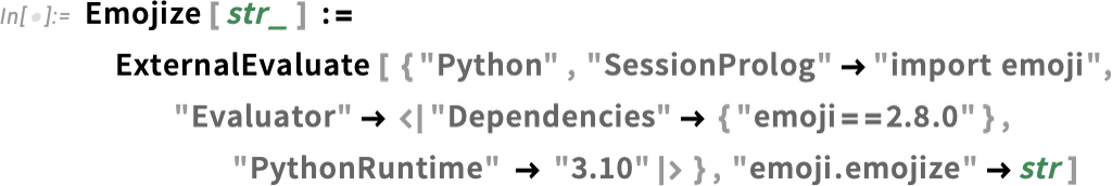
And now you can just call Emojize in the Wolfram Language and—under the hood—it’ll run Python code:
\n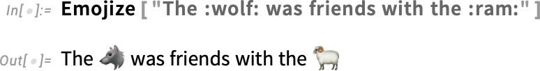
The way this works is that the first time you call Emojize, a Python environment with all the right features is created, then is cached for subsequent uses. And what’s important is that the Wolfram Language specification of Emojize is completely system independent (or as system independent as it can be, given vicissitudes of Python implementations). So that means that you can, for example, deploy Emojize in the Wolfram Function Repository just like you would deploy something written purely in Wolfram Language.
\nThere’s very different engineering involved in calling C-compatible functions in dynamic libraries. But in Version 13.3 we also made this very streamlined using the function ForeignFunctionLoad. There’s all sorts of complexity associated with converting to and from native C data types, managing memory for data structures, etc. But we’ve now got very clean ways to do this in Wolfram Language.
\nAs an example, here’s how one sets up a “foreign function” call to a function RAND_bytes in the OpenSSL library:
\n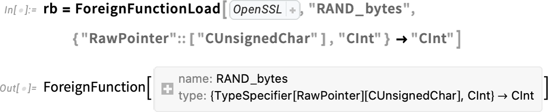
Inside this, we’re using Wolfram Language compiler technology to specify the native C types that will be used in the foreign function. But now we can package this all up into a Wolfram Language function:
\n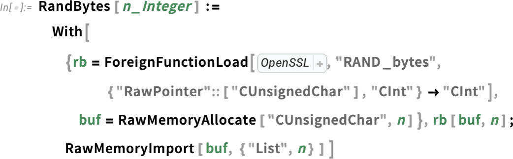
And we can call this function just like any other Wolfram Language function:
\nInternally, all sorts of complicated things are going on. For example, we’re allocating a raw memory buffer that’s then getting fed to our C function. But when we do that memory allocation we’re creating a symbolic structure that defines it as a “managed object”:
\n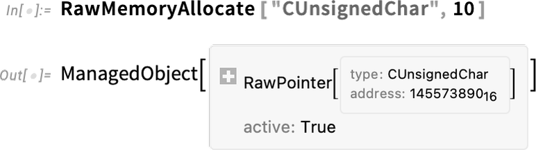
And now when this object is no longer being used, the memory associated with it will be automatically freed.
\nAnd, yes, with both Python and C there’s quite a bit of complexity underneath. But the good news is that in Version 14 we’ve basically been able to automate handling it. And the result is that what gets exposed is pure, simple Wolfram Language.
\nBut there’s another big piece to this. Within particular Python or C libraries there are often elaborate definitions of data structures that are specific to that library. And so to use these libraries one has to dive into all the—potentially idiosyncratic—complexities of those definitions. But in the Wolfram Language we have consistent symbolic representations for things, whether they’re images, or dates or types of chemicals. When you first hook up an external library you have to map its data structures to these. But once that’s done, anyone can use what’s been built, and seamlessly integrate with other things they’re doing, perhaps even calling other external code. In effect what’s happening is that one’s leveraging the whole design framework of the Wolfram Language, and applying that even when one’s using underlying implementations that aren’t based on the Wolfram Language.
\nA single line (or less) of Wolfram Language code can do a lot. But one of the remarkable things about the language is that it’s fundamentally scalable: good both for very short programs and very long programs. And since Version 13 there’ve been several advances in handling very long programs. One of them concerns “code editing”.
\nStandard Wolfram Notebooks work very well for exploratory, expository and many other forms of work. And it’s certainly possible to write large amounts of code in standard notebooks (and, for example, I personally do it). But when one’s doing “software-engineering-style work” it’s both more convenient and more familiar to use what amounts to a pure code editor, largely separate from code execution and exposition. And this is why we have the “package editor”, accessible from File > New > Package/Script. You’re still operating in the notebook environment, with all its sophisticated capabilities. But things have been “skinned” to provide a much more textual “code experience”—both in terms of editing, and in terms of what actually gets saved in .wl files.
\nHere’s typical example of the package editor in action (in this case applied to our GitLink package):
\n
Several things are immediately evident. First, it’s very line oriented. Lines (of code) are numbered, and don’t break except at explicit newlines. There are headings just like in ordinary notebooks, but when the file is saved, they’re stored as comments with a certain stylized structure:
\n 
It’s still perfectly possible to run code in the package editor, but the output won’t get saved in the .wl file:
\n
One thing that’s changed since Version 13 is that the toolbar is much enhanced. And for example there’s now “smart search” that is aware of code structure:
\n
You can also ask to go to a line number—and you’ll immediately see whatever lines of code are nearby:
\n
In addition to code editing, another set of features new since Version 13 of importance to serious developers concern automated testing. The main advance is the introduction of a fully symbolic testing framework, in which individual tests are represented as symbolic objects
\n
and can be manipulated in symbolic form, then run using functions like TestEvaluate and TestReport:
\n
In Version 14.0 there’s another new testing function—IntermediateTest—that lets you insert what amount to checkpoints inside larger tests:
\n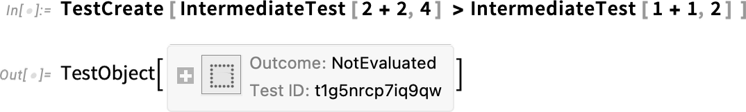
Evaluating this test, we see that the intermediate tests were also run:
\n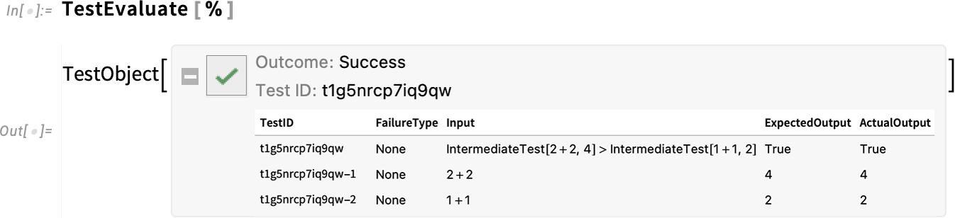
The Wolfram Function Repository has been a big success. We introduced it in 2019 as a way to make specific, individual contributed functions available in the Wolfram Language. And now there are more than 2900 such functions in the Repository.
\nThe nearly 7000 functions that constitute the Wolfram Language as it is today have been painstakingly developed over the past three and a half decades, always mindful of creating a coherent whole with consistent design principles. And now in a sense the success of the Function Repository is one of the dividends of all that effort. Because it’s the coherence and consistency of the underlying language and its design principles that make it feasible to just add one function at a time, and have it really work. You want to add a function to do some very specific operation that combines images and graphs. Well, there’s a consistent representation of both images and graphs in the Wolfram Language, which you can leverage. And by following the principles of the Wolfram Language—like for the naming of functions—you can create a function that’ll be easy for Wolfram Language users to understand and use.
\nUsing the Wolfram Function Repository is a remarkably seamless process. If you know the function’s name, you can just call it using ResourceFunction; the function will be loaded if it’s needed, and then it’ll just run:
\n
If there’s an update available for the function, it’ll give you a message, but run the old version anyway. The message has a button that lets you load in the update; then you can rerun your input and use the new version. (If you’re writing code where you want to “burn in” a particular version of a function, you can just use the ResourceVersion option of ResourceFunction.)
\nIf you want your code to look more elegant, just evaluate the ResourceFunction object
\n
and use the formatted version:
\n
And, by the way, pressing the + then gives you more information about the function:
\n 
An important feature of functions in the Function Repository is that they all have documentation pages—that are organized pretty much like the pages for built-in functions:
\n
But how does one create a Function Repository entry? Just go to File > New > Repository Item > Function Repository Item and you’ll get a Definition Notebook:
\n
We’ve optimized this to be as easy to fill in as possible, minimizing boilerplate and automatically checking for correctness and consistency whenever possible. And the result is that it’s perfectly realistic to create a simple Function Repository item in under an hour—with the main time spent being in the writing of good expository examples.
\nWhen you press Submit to Repository your function gets sent to the Wolfram Function Repository review team, whose mandate is to ensure that functions in the repository do what they say they do, work in a way that is consistent with general Wolfram Language design principles, have good names, and are adequately documented. Except for very specialized functions, the goal is to finish reviews within a week (and sometimes considerably sooner)—and to publish functions as soon as they are ready.
\nThere’s a digest of new (and updated) functions in the Function Repository that gets sent out every Friday—and makes for interesting reading (you can subscribe here):
\n 
The Wolfram Function Repository is a curated public resource that can be accessed from any Wolfram Language system (and, by the way, the source code for every function is available—just press the Source Notebook button). But there’s another important use case for the infrastructure of the Function Repository: privately deployed “resource functions”.
\nIt all works through the Wolfram Cloud. You use the exact same Definition Notebook, but now instead of submitting to the public Wolfram Function Repository, you just deploy your function to the Wolfram Cloud. You can make it private so that only you, or some specific group, can access it. Or you can make it public, so anyone who knows its URL can immediately access and use it in their Wolfram Language system.
\nThis turns out to be a tremendously useful mechanism, both for group projects, and for creating published material. In a sense it’s a very lightweight but robust way to distribute code—packaged into functions that can immediately be used. (By the way, to find the functions you’ve published from your Wolfram Cloud account, just go to the DeployedResources folder in the cloud file browser.)
\n(For organizations that want to manage their own function repository, it’s worth mentioning that the whole Wolfram Function Repository mechanism—including the infrastructure for doing reviews, etc.—is also available in a private form through the Wolfram Enterprise Private Cloud.)
\nSo what’s in the public Wolfram Function Repository? There are a lot of “specialty functions” intended for specific “niche” purposes—but very useful if they’re what you want:
\n


There are functions that add various kinds of visualizations:
\n


Some functions set up user interfaces:
\n
Some functions link to external services:
\n


Some functions provide simple utilities:
\n
There are also functions that are being explored for potential inclusion in the core system:
\n

There are also lots of “leading-edge” functions, added as part of research or exploratory development. And for example in pieces I write (including this one), I make a point of having all pictures and other output be backed by “click-to-copy” code that reproduces them—and this code quite often contains functions either from the public Wolfram Function Repository or from (publicly accessible) private deployments.
\nPaclets are a technology we’ve used for more than a decade and a half to distribute updated functionality to Wolfram Language systems in the field. In Version 13 we began the process of providing tools for anyone to create paclets. And since Version 13 we’ve introduced the Wolfram Language Paclet Repository as a centralized repository for paclets:
\n
What is a paclet? It’s a collection of Wolfram Language functionality—including function definitions, documentation, external libraries, stylesheets, palettes and more—that can be distributed as a unit, and immediately deployed in any Wolfram Language system.
\nThe Paclet Repository is a centralized place where anyone can publish paclets for public distribution. So how does this relate to the Wolfram Function Repository? They are interestingly complementary—with different optimization and different setups. The Function Repository is more lightweight, the Paclet Repository more flexible. The Function Repository is for making available individual new functions, that independently fit into the whole existing structure of the Wolfram Language. The Paclet Repository is for making available larger-scale pieces of functionality, that can define a whole framework and environment of their own.
\nThe Function Repository is also fully curated, with every function being reviewed by our team before it is posted. The Paclet Repository is an immediate-deployment system, without pre-publication review. In the Function Repository every function is specified just by its name—and our review team is responsible for ensuring that names are well chosen and have no conflicts. In the Paclet Repository, every contributor gets their own namespace, and all their functions and other material live inside that namespace. So, for example, I contributed the function RandomHypergraph to the Function Repository, which can be accessed just as ResourceFunction[\"RandomHypergraph\"]. But if I had put this function in a paclet in the Paclet Repository, it would have to be accessed as something like PacletSymbol[\"StephenWolfram/Hypergraphs\", \"RandomHypergraph\"].
\nPacletSymbol, by the way, is a convenient way of “deep accessing” individual functions inside a paclet. PacletSymbol temporarily installs (and loads) a paclet so that you can access a particular symbol in it. But more often one wants to permanently install a paclet (using PacletInstall), then explicitly load its contents (using Needs) whenever one wants to have its symbols available. (All the various ancillary elements, like documentation, stylesheets, etc. in a paclet get set up when it is installed.)
\nWhat does a paclet look like in the Paclet Repository? Every paclet has a home page that typically includes an overall summary, a guide to the functions in the paclet, and some overall examples of the paclet:
\n
Individual functions typically have their own documentation pages:
\n 
Just like in the main Wolfram Language documentation, there can be a whole hierarchy of guide pages, and there can be things like tutorials.
\nNotice that in examples in paclet documentation, one often sees constructs like ![]() . These represent symbols in the paclet, presented in forms like PacletSymbol[\"WolframChemistry/ProteinVisualization\", \"AmidePlanePlot\"] that allow these symbols to be accessed in a “standalone” way. If you directly evaluate such a form, by the way, it’ll force (temporary) installation of the paclet, then return the actual, raw symbol that appears in the paclet:
. These represent symbols in the paclet, presented in forms like PacletSymbol[\"WolframChemistry/ProteinVisualization\", \"AmidePlanePlot\"] that allow these symbols to be accessed in a “standalone” way. If you directly evaluate such a form, by the way, it’ll force (temporary) installation of the paclet, then return the actual, raw symbol that appears in the paclet:
So how does one create a paclet suitable for submission to the Paclet Repository? You can do it purely programmatically, or you can start from File > New > Repository Item > Paclet Repository Item, which launches what amounts to a whole paclet creation IDE. The first step is to specify where you want to assemble your paclet. You give some basic information
\n
then a Paclet Resource Definition Notebook is created, from which you can give function definitions, set up documentation pages, specify what you want your paclet’s home page to be like, etc.:
\n
There are lots of sophisticated tools that let you create full-featured paclets with the same kind of breadth and depth of capabilities that you find in the Wolfram Language itself. For example, Documentation Tools lets you construct full-featured documentation pages (function pages, guide pages, tutorials, …):
\n
Once you’ve assembled a paclet, you can check it, build it, deploy it privately—or submit it to the Paclet Repository. And once you submit it, it will automatically get set up on the Paclet Repository servers, and within just a few minutes the pages you’ve created describing your paclet will show up on the Paclet Repository website.
\nSo what’s in the Paclet Repository so far? There’s a lot of good and very serious stuff, contributed both by teams at our company and by members of the broader Wolfram Language community. In fact, many of the 134 paclets now in the Paclet Repository have enough in them that there’s a whole piece like this that one could write about them.
\nOne category of things you’ll find in the Paclet Repository are snapshots of our ongoing internal development projects—many of which will eventually become built-in parts of the Wolfram Language. A good example of this is our LLM and Chat Notebook functionality, whose rapid development and deployment over the past year was made possible by the use of the Paclet Repository. Another example, representing ongoing work from our chemistry team (AKA WolframChemistry in the Paclet Repository) is the ChemistryFunctions paclet, which contains functions like:
\n
And, yes, this is interactive:
\n
Or, also from WolframChemistry:
\n
Another “development snapshot” is DiffTools—a paclet for making and viewing diffs between strings, cells, notebooks, etc.:
\n
A major paclet is QuantumFramework—which provides the functionality for our Wolfram Quantum Framework
\n
and delivers broad support for quantum computing (with at least a few connections to multiway systems and our Physics Project):
\n

Talking of our Physics Project, there are over 200 functions supporting it that are in the Wolfram Function Repository. But there are also paclets, like WolframInstitute/Hypergraph:
\n
An example of an externally contributed package is Automata—with more than 250 functions for doing computations related to finite automata:
\n

Another contributed paclet is FunctionalParsers, which goes from a symbolic parser specification to an actual parser, here being used in a reverse mode to generate random “sentences”:
\n
Phi4Tools is a more specialized paclet, for working with Feynman diagrams in ![]() field theory:
field theory:


And, as another example, here’s MaXrd, for crystallography and x-ray scattering:
\n

As just one more example, there’s the Organizer paclet—a utility paclet for making and manipulating organizer notebooks. But unlike the other paclets we’ve seen here, it doesn’t expose any Wolfram Language functions; instead, when you install it, it puts a palette in your Palettes list:
\n

As of today, Version 14 is finished, and out in the world. So what’s next? We have lots of projects underway—some already with years of development behind them. Some extend and strengthen what’s already in the Wolfram Language; some take it in new directions.
\nOne major focus is broadening and streamlining the deployment of the language: unifying the way it’s delivered and installed on computers, packaging it so it can be efficiently integrated into other standalone applications, etc.
\nAnother major focus is expanding the handling of very large amounts of data by the Wolfram Language—and seamlessly integrating out-of-core and lazy processing.
\nThen of course there’s algorithmic development. Some is “classical”, directly building on the towers of functionality we’ve developed over the decades. Some is more “AI based”. We’ve been creating heuristic algorithms and meta-algorithms ever since Version 1.0—increasingly using methods from machine learning. How far will neural net methods go? We don’t know yet. We’re routinely using them in things like algorithm selection. But to what extent can they help in the heart of algorithms?
\nI’m reminded of something we did back in 1987 in developing Version 1.0. There was a long tradition in numerical analysis of painstakingly deriving series approximations for particular cases of mathematical functions. But we wanted to be able to compute hundreds of different functions to arbitrary precision for any complex values of their arguments. So how did we do it? We generalized from series to rational approximations—and then, in a very “machine-learning-esque” way—we spent months of CPU time systematically optimizing these approximations. Well, we’ve been trying to do the same kind of thing again—though now over more ambitious domains—and now using not rational functions but large neural nets as our basis.
\nWe’ve also been exploring using neural nets to “control” precise algorithms, in effect making heuristic choices which either guide or can be validated by the precise algorithms. So far, none of what we’ve produced has outperformed our existing methods, but it seems plausible that fairly soon it will.
\nWe’re doing a lot with various aspects of metaprogramming. There’s the project of
\ngetting LLMs to help in the construction of Wolfram Language code—and in giving comments on it, and in analyzing what went wrong if the code didn’t do what one expected. Then there’s code annotation—where LLMs may help in doing things like predicting the most likely type for something. And there’s code compilation. We’ve been working for many years on a full-scale compiler for the Wolfram Language, and in every version what we have becomes progressively more capable. We’ve been doing some level of automatic compilation in particular cases (particularly ones involving numerical computation) for more than 30 years. And eventually full-scale automatic compilation will be possible for everything. But as of now some of the biggest payoffs from our compiler technology have been for our internal development, where we can now get optimal down-to-the-metal performance simply by compiled (albeit carefully written) Wolfram Language code.
One of the big lessons of the surprising success of LLMs is that there’s potentially more structure in meaningful human language than we thought. I’ve long been interested in creating what I’ve called a “symbolic discourse language” that gives a computational representation of everyday discourse. The LLMs haven’t explicitly done that. But they encourage the idea that it should be possible, and they also provide practical help in doing it. And whether the goal is to be able to represent narrative text, or contracts, or textual specifications, it’s a matter of extending the computational language we’ve built to encompass more kinds of concepts and structures.
\nThere are typically several kinds of drivers for our continued development efforts. Sometimes it’s a question of continuing to build a tower of capabilities in some known direction (like, for example, solving PDEs). Sometimes the tower we’ve built suddenly lets us see new possibilities. Sometimes when we actually use what we’ve built we realize there’s an obvious way to polish or extend it—or to “double down” on something that we can now see is valuable. And then there are cases where things happening in the technology world suddenly open up new possibilities—like LLMs have recently done, and perhaps XR will eventually do. And finally there are cases where new science-related insights suggest new directions.
\nI had assumed that our Physics Project would at best have practical applications only centuries hence. But in fact it’s become clear that the correspondence it’s defined between physics and computation gives us quite immediate new ways to think about aspects of practical computation. And indeed we’re now actively exploring how to use this to define a new level of parallel and distributed computation in the Wolfram Language, as well as to represent symbolically not only the results of computations but also the ongoing process of computation.
\nOne might think that after nearly four decades of intense development there wouldn’t be anything left to do in developing the Wolfram Language. But in fact at every level we reach, there’s ever more that becomes possible, and ever more that can we see might be possible. And indeed this moment is a particularly fertile one, with an unprecedentedly broad waterfront of possibilities. Version 14 is an important and satisfying waypoint. But there are wonderful things ahead—as we continue our long-term mission to make the computational paradigm achieve its potential, and to build our computational language to help that happen.
\n\n\n\n
\n", "category": "Big Picture", "link": "https://writings.stephenwolfram.com/2024/01/the-story-continues-announcing-version-14-of-wolfram-language-and-mathematica/", "creator": "Stephen Wolfram", "pubDate": "Tue, 09 Jan 2024 22:33:01 +0000", "enclosure": "https://content.wolfram.com/sites/43/2024/01/stream-plot-small.mp4", "enclosureType": "video/mp4", "image": "https://content.wolfram.com/sites/43/2024/01/stream-plot-small.mp4", "id": "", "language": "en", "folder": "", "feed": "wolfram", "read": false, "favorite": false, "created": false, "tags": [], "hash": "8e9ed31ddb65ef517482505f1b29daef", "highlights": [] }, { "title": "Observer Theory", "description": "
We call it perception. We call it measurement. We call it analysis. But in the end it’s about how we take the world as it is, and derive from it the impression of it that we have in our minds.
\nWe might have thought that we could do science “purely objectively” without any reference to observers or their nature. But what we’ve discovered particularly dramatically in our Physics Project is that the nature of us as observers is critical even in determining the most fundamental laws we attribute to the universe.
\nBut what ultimately does an observer—say like us—do? And how can we make a theoretical framework for it? Much as we have a general model for the process of computation—instantiated by something like a Turing machine—we’d like to have a general model for the process of observation: a general “observer theory”.
\nCentral to what we think of as an observer is the notion that the observer will take the raw complexity of the world and extract from it some reduced representation suitable for a finite mind. There might be zillions of photons impinging on our eyes, but all we extract is the arrangement of objects in a visual scene. Or there might be zillions of gas molecules impinging on a piston, yet all we extract is the overall pressure of the gas.
\nIn the end, we can think of it fundamentally as being about equivalencing. There are immense numbers of different individual configurations for the photons or the gas molecules—that are all treated as equivalent by an observer who’s just picking out the particular features needed for some reduced representation.
\nThere’s in a sense a certain duality between computation and observation. In computation one’s generating new states of a system. In observation, one’s equivalencing together different states.
\nThat equivalencing must in the end be implemented “underneath” by computation. But in observer theory what we want to do is just characterize the equivalencing that’s achieved. For us as observers it might in practice be all about how our senses work, what our biological or cultural nature is—or what technological devices or structures we’ve built. But what makes a coherent concept of observer theory possible is that there seem to be general, abstract characterizations that capture the essence of different kinds of observers.
\nIt’s not immediately obvious that anything suitable for a finite mind could ever be extracted from the complexity of the world. And indeed the Principle of Computational Equivalence implies that computational irreducibility (and its multicomputational generalization) will be ubiquitous. But within computational irreducibility there must always be slices of computational reducibility. And it’s these slices of reducibility that an observer must try to pick out—and that ultimately make it possible for a finite mind to develop a “useful narrative” about what happens in the world, that allows it to make decisions, predictions, and so on.
\nHow “special” is what an observer does? At its core it’s just about taking a large set of possible inputs, and returning a much smaller set of possible outputs. And certainly that’s a conceptual idea that’s appeared in many fields under many different names: a contractive mapping, reduction to canonical form, a classifier, an acceptor, a forgetful functor, evolving to an attractor, extracting statistics, model fitting, lossy compression, projection, phase transitions, renormalization group transformations, coarse graining and so on. But here we want to think not about what’s “mathematically describable”, but instead about what in general is actually implemented—say by our senses, our measuring devices, or our ways of analyzing things.
\nAt an ultimate level, everything that happens can be thought of as being captured by the ruliad—the unique object that emerges as the entangled limit of all possible computations. And in a vast generalization of ideas like that our brains—like any other material thing—are made of atoms, so too any observer must be embedded as some kind of structure within the ruliad. But a key concept of observer theory is that it’s possible to make conclusions about an observer’s impression of the world just by knowing about the capabilities—and assumptions—of the observer, without knowing in detail what the observer is “like inside”.
\nAnd so it is, for example, that in our Physics Project we seem to be able to derive—essentially from the structure of the ruliad—the core laws of twentieth-century physics (general relativity, quantum mechanics and the Second Law) just on the basis of two features of us as observers: that we’re computationally bounded, and that we believe we’re persistent in time (even though “underneath” we’re made of different atoms of space at every successive moment). And we can expect that if we were to include other features of us as observers (for example, that we believe there are persistent objects in the world, or that we believe we have free will) then we’d be able to derive more aspects of the universe as we experience it—or of natural laws we attribute to it.
\nBut the notion of observers—and observer theory—isn’t limited purely to “physical observers”. It applies whenever we try to “get an impression” of something. And so, for example, we can also operate as “mathematical observers”, sampling the ruliad to build up conclusions about mathematical laws. Some features of us as physical observers—like the computational boundedness associated with the finiteness of our minds—inevitably carry over to us as mathematical observers. But other features do not. But the point of observer theory is to provide a general framework in which we can characterize observers—and then see the consequences of those characterizations for the impressions or conclusions observers will form.
\n
As humans we have senses like sight, hearing, touch, taste, smell and balance. And through our technology we also have access to a few thousand other kinds of measurements. So how basically do all these work?
\nThe vast majority in effect aggregate a large number of small inputs to generate some kind of “average” output—which in the case of measurements is often specified as a (real) number. In a few cases, however, there’s instead a discrete choice between outputs that’s made on the basis of whether the total input exceeds a threshold (think: distributed consensus schemes, weighing balances, etc.)
\nBut in all cases what’s fundamentally happening is that lots of different input configurations are all being equivalenced—or, more operationally, the dynamics of the system essentially make all equivalenced states evolve to the same “attractor state”.
\nAs an example, let’s consider measuring the pressure of a gas. There are various ways to do this. But a very direct one is just to have a piston, and see how much force is exerted by the gas on this piston. So where does this force come from? At the lowest level it’s the result of lots of individual molecules bouncing off the surface of the piston, each transferring a tiny amount of momentum to it. If we looked at the piston at an atomic scale, we’d see it temporarily deform from each molecular impact. But the crucial point is that at a large scale the piston moves together, as a single rigid object—aggregating the effects of all those individual molecular impacts.
\nBut why does it work this way? Essentially it’s because the intermolecular forces inside the piston are much stronger than the forces associated with molecules in the gas. Or, put more abstractly, there’s more coupling and coherence “inside the observer” than between the observer and what it’s observing.
\nWe see the same basic pattern over and over again. There’s some form of transduction that couples the individual elements of what’s being observed to the observer. Then “within the observer” there’s something that in essence aggregates all these small effects. Sometimes that aggregation is “directly numerical”, as in the addition of lots of small momentum transfers. But sometimes it’s instead more explicitly like evolution to one attractor rather than another.
\nConsider, for example, the case of vision. An array of photons fall on the photoreceptor cells on our retinas, generating electrical signals transmitted through nerve fibers to our brains. Within the brain there’s then effectively a neural net that evolves to different attractors depending on what one’s looking at. Most of the time a small change in input image won’t affect what attractor one evolves to. But—much like with a weighing balance—there’s an “edge” at which even a small change can lead to a different output.
\nOne can go through lots of different types of sensory systems and measuring devices. But the basic outline seems to always be the same. First, there’s a coupling between what is being sensed or measured and the thing that’s doing the sensing or measuring. Quite often that coupling involves transducing from one physical form to another—say from light to electricity, or from force to position. Sometimes then the crucial step of equivalencing different detailed inputs is achieved by simple “numerical aggregation”, most often by accumulation of objects (atoms, raindrops, etc.) or physical effects (forces, currents, etc.). But sometimes the equivalencing is instead achieved by a more obviously dynamical process.
\nIt could amount to simple amplification, in which, say, the presence of a small element of input (say an individual particle) “tips over” some metastable system so that it goes into a certain final state. Or it could be more like a neural net where there’s a more complicated translation defined by hard-to-describe borders between basins of attraction leading to different attractors.
\nBut, OK, so what’s the endpoint of a process of observation? Ultimately for us humans it’s an impression created in our minds. Of course that gets into lots of slippery philosophical issues. Yes, each of us has an “inner experience” of what’s going on in our mind. But anything else is ultimately an extrapolation. We make the assumption that other human minds also “see what we see”, but we can never “feel it from the inside”.
\nWe can of course make increasingly detailed measurements—say of neural activity—to see how similar what’s going on is between one brain and another. But as soon as there’s the slightest structural—or situational—difference between the brains, we really can’t say exactly how their “impressions” will compare.
\nBut for our purposes in constructing a general “observer theory” we’re basically going to make the assumption (or, in effect, “philosophical approximation”) that whenever a system does enough equivalencing, that’s tantamount to it “acting like an observer”, because it can then act as a “front end” that takes the “incoherent complexity of the world” and “collimates it” to the point where a mind will derive a definite impression from it.
\nOf course, there’s still a lot of subtlety here. There has to be “just enough equivalencing” and not too much. For example, if all inputs were always equivalenced to the same output, there’d be nothing useful observed. And in the end there’s somehow got to be some kind of match between the compression of input achieved by equivalencing, and the “capacity” of the mind that’s ultimately deriving an impression from it.
\nA crucial feature of anything that can reasonably be called a mind is that “something’s got to be going on in there”. It can’t be, for example, that the internal state of the system is fixed. There has to be some internal dynamics—some computational process that we can identify as the ongoing operation of the mind.
\nAt an informational level we might say that there has to be more information processing going on inside than there is flow of information from the outside. Or, in other words, if we’re going to be meaningful “observers like us” we can’t just be bombarded by input we don’t process; we have to have some capability to “think about what we’re seeing”.
\nAll of this comes back to the idea that a crucial feature of us as observers is that we are computationally bounded. We do computation; that’s why we can have an “inner sense of things going on”. But the amount of computation we do is tiny compared to the computation going on in the world around us. Our experience represents a heavily filtered version of “what’s happening outside”. And the essence of “being an observer like us” is that we’re effectively doing lots of equivalencing to get to that filtered version.
\nBut can we imagine a future in which we “expand our minds”? Or perhaps encounter some alien intelligence with a fundamentally “less constrained mind”? Well, at some point there’s an issue with this. Because in a sense the idea that we have a coherent existence relies on us having “limited minds”. For without such constraints there wouldn’t be a coherent “self” that we could identify—with coherent inner experience.
\nLet’s say we’re shown some system—say in nature—“from the outside”. Can we tell if “there’s an observer in there”? Ultimately not, because in a sense we’d have to be “inside that observer” and be able to experience the impression of the world that it’s getting. But in much the same way as we extrapolate to believing that, say, other human minds are experiencing things like we’re experiencing, so also we can potentially extrapolate to say what we might think of as an observer.
\nAnd the core idea seems to be that an “observer” should be a subsystem whose “internal states” are affected by the rest of the system, but where many “external states” lead to the same internal state—and where there is rich dynamics “within the observer” that in effect operates only on its internal states. Ultimately—following the Principle of Computational Equivalence—both the outside and the inside of the “observer subsystem” can be expected to be equivalent in the computations they’re performing. But the point is that the coupling from outside the subsystem to inside effectively “coarse grains” what’s outside, so that the “inner computation” is operating on a much-reduced set of elements.
\nWhy should any such “observer subsystems” exist? Presumably at some level it’s inevitable from the presence of pockets of computational reducibility within arbitrary computationally irreducible systems. But more important for us is that our very existence—and the possibility of our coherent inner experience—depends on us “operating as observers”. And—almost as a “self-fulfilling prophecy”—our behavior tends to perpetuate our ability to successfully do this. For example, we can think of us as choosing to put ourselves in situations and environments where we can “predict what’s going to happen” well enough to “survive as observers”. (At a mundane practical level we might do this by not living in places subject to unpredictable natural forces—or by doing things like building ourselves structures that shelter us from those forces.)
\nWe’ve talked about observers operating by compressing the complexities of the world to “inner impressions” suitable for finite minds. And in typical situations that we describe as perception and measurement, the main way this happens is by fairly direct equivalencing of different states. But in a sense there’s a higher-level story that relies on formalization—and in essence computation—and that’s what we usually call “analysis”.
\nLet’s say we have some intricate structure—perhaps some nested, fractal pattern. A direct rendering of all the pixels in this pattern ultimately won’t be something well suited for a “finite mind”. But if we gave rules—or a program—for generating the pattern we’d have a much more succinct representation of it.
\nBut now there’s a problem with computational irreducibility. Yes, the rules determine the pattern. But to get from these rules to the actual pattern can require an irreducible amount of computation. And to “reverse engineer the pattern” to find the rules can require even more computation.
\nYes, there are particular cases—like repetitive and simple nested patterns—where there’s enough immediate computational reducibility that a computationally bounded system (or observer) can fairly easily “do the analysis” and “get the compression”. But in general it’s hard. And indeed in a sense it’s the whole mission of science to pick away at the problem, and try to find more ways to “reduce the complexities of the world” to “human-level narratives”.
\nComputational irreducibility limits the extent to which this can be successful. But the inevitable existence of pockets of reducibility even within computational irreducibility guarantees that progress can always in principle be made. As we invent more kinds of measuring devices we can extend our domain as observers. And the same is true when we invent more methods of analysis, or identify more principles in science.
\nBut the overall picture remains the same: what’s crucial to “being an observer” is equivalencing many “states of the world”, either through perceiving or measuring only specific aspects of them, or through identifying “simplified narratives” that capture them. (In effect, perception and measurement tend to do “lossy compression”; analysis is more about “lossless compression” where the equivalencing is effectively not between possible inputs but between possible generative rules.)
\n
Our view of the world is ultimately determined by what we observe of it. We take what’s “out there in the world” and in effect “construct our perceived reality” by our operation as observers. Or, in other words, insofar as we have a narrative about “what’s going on in the world”, that’s something that comes from our operation as observers.
\nAnd in fact from our Physics Project we’re led to an extreme version of this—in which what’s “out there in the world” is just the whole ruliad, and in effect everything specific about our perceived reality must come from how we operate as observers and thus how we sample the ruliad.
\nBut long before we get to this ultimate level of abstraction, there are lots of ways in which our nature as observers “builds” our perceived reality. Think about any material substance—like a fluid. Ultimately it’s made up of lots of individual molecules “doing their thing”. But observers like us aren’t seeing those molecules. Instead, we’re aggregating things to the point where we can just describe the system as a fluid, that operates according to the “narrative” defined by the laws of fluid mechanics.
\nBut why do things work this way? Ultimately it’s the result of the repeated story of the interplay between underlying computational irreducibility, and the computational boundedness of us as observers. At the lowest level the motion of the molecules is governed by simple rules of mechanics. But the phenomenon of computational irreducibility implies that to work out the detailed consequences of “running these rules” involves an irreducible amount of computational work—which is something that we as computationally bounded observers can’t do. And the result of this is that we’ll end up describing the detailed behavior of the molecules as just “random”. As I’ve discussed at length elsewhere, this is the fundamental origin of the Second Law of thermodynamics. But for our purposes here the important point is that it’s what makes observers like us “construct the reality” of things like fluids. Our computational boundedness as observers makes us unable to trace all the detailed behavior of molecules, and leaves us “content” to describe fluids in terms of the “narrative” defined by the laws of fluid mechanics.
\nOur Physics Project implies that it’s the same kind of story with physical space. For in our Physics Project, space is ultimately “made” of a network of relations (or connections) between discrete “atoms of space”—that’s progressively being updated in what ends up being a computationally irreducible way. But we as computationally bounded observers can’t “decode” all the details of what’s happening, and instead we end up with a simple “aggregate” narrative, that turns out to correspond to continuum space operating according to the laws of general relativity.
\nThe way both coherent notions of “matter” (or fluids) and spacetime emerge for us as observers can be thought of as a consequence of the equivalencing we do as observers. In both cases, there’s immense and computationally irreducible complexity “underneath”. But we’re ignoring most of that—by effectively treating different detailed behaviors as equivalent—so that in the end we get to a (comparatively) “simple narrative” more suitable for our finite minds. But we should emphasize that what’s “really going on in the system” is something much more complicated; it’s just that we as observers aren’t paying attention to that, so our perceived reality is much simpler.
\nOK, but what about quantum mechanics? In a sense that’s an extreme test of our description of how observers work, and the extent to which the operation of observers “constructs their perceived reality”.
\n
In our Physics Project the underlying structure (hypergraph) that represents space and everything in it is progressively being rewritten according to definite rules. But the crucial point is that at any given stage there can be lots of ways this rewriting can happen. And the result is that there’s a whole tree of possible “states of the universe” that can be generated. So given this, why do we ever think that definite things happen in the universe? Why don’t we just think that there’s an infinite tree of branching histories for the universe?
\nWell, it all has to do with our nature as observers, and the equivalencing we do. At an immediate level, we can imagine looking at all those different possible branching paths for the evolution of the universe. And the key point is that even though they come from different paths of history, two states can just be the same. Sometimes it’ll be obvious that they’re same; sometimes one might have to determine, say, whether two hypergraphs are isomorphic. But the point is that to any observer (at least one that isn’t managing to look at arbitrary “implementation details”), the states will inevitably be considered equivalent.
\nBut now there’s a bigger point. Even though “from the outside” there might be a whole branching and merging multiway graph of histories for the universe, observers like us can’t trace that. And in fact all we perceive is a single thread of history. Or, said another way, we believe that we have a single thread of experience—something closely related to our belief that (despite the changing “underlying elements” from which we are made) we are somehow persistent in time (at least during the span of our existence).
\nBut operationally, how do we go from all those underlying branches of history to our perceived single thread of history? We can think of the states on different threads of history as being related by what we call a branchial graph, that joins states that have immediate common ancestors. And in the limit of many threads, we can think of these different states as being laid out “branchial space”. (In traditional quantum mechanics terms, this layout defines a “map of quantum entanglements”—with each piece of common ancestry representing an entanglement between states.)
\nIn physical space—whether we’re looking at molecules in a fluid or atoms of space—we can think of us operating as observers who are physically large enough to span many underlying discrete elements, so that what we end up observing is just some kind of aggregate, averaged result. And it’s very much the same kind of thing in branchial space: we as observers tend to be large enough in branchial space to be spread across an immense number of branches of history, so that what we observe is just aggregate, averaged results across all those branches.
\nThere’s lots of detailed complexity in what happens on different branches, just like there is in what happens to different molecules, or different atoms of space. And the reason is that there’s inevitably computational irreducibility, or, in this case, more accurately, multicomputational irreducibility. But as computationally bounded observers we just perceive aggregate results that “average out” the “underlying apparent randomness” to give a consistent single thread of experience.
\nAnd effectively this is what happens in the transition from quantum to classical behavior. Even though there are many possible detailed (“quantum”) threads of history that an object can follow, what we perceive corresponds to a single consistent “aggregate” (“classical”) sequence of behavior.
\nAnd this is typically true even at the level of our typical observation of molecules and chemical processes. Yes, there are many possible threads of history for, say, a water molecule. But most of our observations aggregate things to the point where we can talk about a definite shape for the molecule, with definite “chemical bonds”, etc.
\nBut there is a special situation that actually looms large in typical discussions of quantum mechanics. We can think of it as the result of doing measurements that aren’t “aggregating threads of history to get an average”, but are instead doing something more like a weighing balance, always “tipping” one way or the other. In the language of quantum computing, we might say that we’re arranging things to be able to “measure a single qubit”. In terms of the equivalencing of states, we might say that we’re equivalencing lots of underlying states to specific canonical states (like “spin up” and “spin down”).
\nWhy do we get one outcome rather than another? Ultimately we can think of it as all depending on the details of us as observers. To see this, let’s start from the corresponding question in physical space. We might ask why we observe some particular thing happening. Well, in our Physics Project everything about “what happens” is deterministic. But there’s still the “arbitrariness” of where we are in physical space. We’ll always basically see the same laws of physics, but the particulars of what we’ll observe depend on where we are, say on the surface of the Earth versus in interstellar space, etc.
\nIs there a “theory” for “where we are”? In some sense, yes, because we can go back and see why the molecules that make us up landed up in the particular place where they did. But what we can’t have an “external theory” for is just which molecules end up making up “us”, as we experience ourselves “from inside”. In our view of physics and the universe, it’s in some sense the only “ultimately subjective” thing: where our internal experience is “situated”.
\nAnd the point is that basically—even though it’s much less familiar—the same thing is going on at the level of quantum mechanics. Just as we “happen” to be at a certain place in physical space, so we’re at a certain place in branchial space. Looking back we can trace how we got here. But there’s no a priori way to determine “where our particular experience will be situated”. And that means we can’t know what the “local branchial environment” will be—and so, for example, what the outcome of “balance-like” measurements will be.
\nJust as in traditional discussions of quantum mechanics, the mechanics of doing the measurement—which we can think of as effectively equivalencing many underlying branches of history—will have an effect on subsequent behavior, and subsequent measurements.
\nBut let’s say we look just at the level of the underlying multiway graph—or, more specifically, the multiway causal graph that records causal connections between different updating events. Then we can identify a complicated web of interdependence between events that are timelike, spacelike and branchlike separated. And this interdependence seems to correspond precisely to what’s expected from quantum mechanics.
\nIn other words, even though the multiway graph is completely determined, the arbitrariness of “where the observer is” (particularly in branchial space), combined with the inevitable interdependence of different aspects of the multiway (causal) graph, seems sufficient to reproduce the not-quite-purely-probabilistic features of quantum mechanics.
\nIn making observations in physical space, it’s common to make a measurement at one place or time, then make another measurement at another place or time, and, for example, see how they’re related. But in actually doing this, the observer will have to move from one place to the other, and persist from one time to another. And in the abstract it’s not obvious that that’s possible. For example, it could be that an observer won’t be able to move without changing—or, in other words, that “pure motion” won’t be possible for an observer. But in effect this is something we as observers assume about ourselves. And indeed, as I’ve discussed elsewhere, this is a crucial part of why we perceive spacetime to operate according to the laws of physics we know.
\nBut what about in branchial space? We have much less intuition for this than for physical space. But we still effectively believe that pure motion is possible for us as observers in branchial space. It could be—like an observer in physical space, say, near a spacetime singularity—that an observer would get “shredded” when trying to “move” in branchial space. But our belief is that typically nothing like that happens. At some level being at different locations in branchial space presumably corresponds to picking different bases for our quantum states, or effectively to defining our experiments differently. And somehow our belief in the possibility of pure motion in branchial space seems related to our belief in the possibility of making arbitrary sequences choices in sets of experiments we do.
\n
We might have thought that the only thing ultimately “out there” for us to observe would be our physical universe. But actually there are important situations where we’re essentially operating not as observers of our familiar physical universe, but instead of what amount to abstract universes. And what we’ll see is that the ideas of observer theory seem to apply there too—except that now what we’re picking out and reducing to “internal impressions” are features not of the physical world but of abstract worlds.
\nOur Physics Project in a sense brings ideas about the physical and abstract worlds closer—and the concept of the ruliad ultimately leads to a deep unification between them. For what we now imagine is that the physical universe as we perceive it is just the result of the particular kind of sampling of the ruliad made by us as certain kinds of observers. And the point is that we as observers can make other kinds of samplings, leading to what we can describe as abstract universes. And one particularly prominent example of this is mathematics, or rather, metamathematics.
\nImagine starting from all possible axioms for mathematics, then constructing the network of all possible theorems that can be derived from them. We can consider this as forming a kind of “metamathematical universe”. And the particular mathematics that some mathematician might study we can then think of as the result of a “mathematical observer” observing that metamathematical universe.
\nThere are both close analogies and differences between this and the experience of a physical observer in the physical universe. Both ultimately correspond to samplings of the ruliad, but somewhat different ones.
\nIn our Physics Project we imagine that physical space and everything in it is ultimately made up of discrete elements that we identify as “atoms of space”. But in the ruliad in general we can think of everything being made up of “pure atoms of existence” that we call emes. In the particular case of physics we interpret these emes as atoms of space. But in metamathematics we can think of emes as corresponding to (“subaxiomatic”) elements of symbolic structures—from which things like axioms or theorems can be constructed.
\nA central feature of our interaction with the ruliad for physics is that observers like us don’t track the detailed behavior of all the various atoms of space. Instead, we equivalence things to the point where we get descriptions that are reduced enough to “fit in our minds”. And something similar is going on in mathematics.
\nWe don’t track all the individual subaxiomatic emes—or usually in practice even the details of fully formalized axioms and theorems. Instead, mathematics typically operates at a much higher and “more human” level, dealing not with questions like how real numbers can be built from emes—or even axioms—but rather with what can be deduced about the properties of mathematical objects like real numbers. In a physics analogy to the behavior of a gas, typical human mathematics operates not at the “molecular” level of individual emes (or even axioms) but rather at the “fluid dynamics” level of “human-accessible” mathematical concepts.
\nIn effect, therefore, a mathematician is operating as an observer who equivalences many detailed configurations—ultimately of emes—in order to form higher-level mathematical constructs suitable for our computationally bounded minds. And while at the outset one might have imagined that anything in the ruliad could serve as a “possible mathematics”, the point is that observers like us can only sample the ruliad in particular ways—leading to only particular possible forms for “human-accessible” mathematics.
\nIt’s a very similar story to the one we’ve encountered many times in thinking about physics. In studying gases, for example, we could imagine all sorts of theories based on tracking detailed molecular motions. But for observers like us—with our computational boundedness—we inevitably end up with things like the Second Law of thermodynamics, and the laws of fluid mechanics. And in mathematics the main thing we end up with is “higher-level mathematics”—mathematics that we can do directly in terms of typical textbook concepts, rather than constantly having to “drill down” to the level of axioms, or emes.
\nIn physics we’re usually particularly concerned with issues like predicting how things will evolve through time. In mathematics it’s more about accumulating what can be considered true. And indeed we can think of an idealized mathematician as going through the ruliad and collecting in their minds a “bag” of theorems (or axioms) that they “consider to be true”. And given such a collection, they can essentially follow the “entailment paths” defined by computations in the ruliad to find more theorems to “add to their bag”. (And, yes, if they put in a false theorem then—because a false premise in the standard setup of logic implies everything—they’ll end up with an “infinite explosion of theorems”, that won’t fit in a finite mind.)
\nIn observing the physical universe, we talk about our different possible senses (like vision, hearing, etc.) or different kinds of measuring devices. In observing the metamathematical universe the analogy is basically different possible kinds of theories or abstractions—say, algebraic vs. geometrical vs. topological vs. categorical, etc. (with new approaches being like new kinds of measuring devices).
\nParticularly when we think in terms of the ruliad we can expect a certain kind of ultimate unity in the metamathematical universe—but different theories and different abstractions will pick up different aspects of it, just as vision and hearing pick up different aspects of the physical universe. But in a sense observer theory gives us a global way to talk about this, and to characterize what kinds of observations observers like us can make—whether of the physical universe or the metamathematical one.
\nIn physics we’ve then seen in our Physics Project how this allows us to find general laws that describe our perception of the physical world—and that turn out to reproduce the core known laws of physics. In mathematics we’re not as familiar with the concept of general laws, though the very fact that higher-level mathematics is possible is presumably in essence such a law, and perhaps the kinds of regularities seen in areas like category theory are others—as are the inevitable dualities we expect to be able to identify between different fields of mathematics. All these laws ultimately rely on the structure of the ruliad. But the crucial point is that they’re not talking about the “raw ruliad”; instead they’re talking about just certain samplings of the ruliad that can be done by observers like us, and that lead to certain kinds of “internal impressions” in terms of which these laws can be stated.
\nMathematics represents a certain kind of abstract setup that’s been studied in a particularly detailed way over the centuries. But it’s not the only kind of “abstract setup” we can imagine. And indeed there’s even a much more familiar one: the use of concepts—and words—in human thinking and language.
\nWe might imagine that at some time in the distant past our forebears could signify, say, rocks only by pointing at individual ones. But then there emerged the general notion of “rock”, captured by a word for “rock”. And once again this is a story of observers and equivalences. When we look at a rock, it presumably produces all sorts of detailed patterns of neuron firings in our brains, different for each particular rock. But somehow—presumably essentially through evolution to an attractor in the neural net in our brains—we equivalence all these patterns to extract our “inner impression” of the “concept of a rock”.
\nIn the typical tradition of quantitative science we tend to be interested in doing measurements that lead to things like numerical results. But in representing the world using language we tend to be interested instead in creating symbolic structures that involve collections of discrete words embedded in a grammatical framework. Such linguistic descriptions don’t capture every detail; in a typical observer kind of way they broadly equivalence many things—and in a sense reduce the complexity of the world to a description in terms of a limited number of discrete words and linguistic forms.
\nWithin any given person’s brain there’ll be “thoughts” defined by patterns of neuron firings. And the crucial role of language is to provide a way to robustly “package up” those thoughts, and for example represent them with discrete words, so they can be communicated to another person—and unpacked in that person’s brain to produce neuron firings that reproduce what amount to those same thoughts.
\nWhen we’re dealing with something like a numerical measurement we might imagine that it could have some kind of absolute interpretation. But words are much more obviously an “arbitrary basis” for communication. We could pick a different specific word (say from a different human language) but still “communicate the same thing”. All that’s required is that everyone who’s using the word agrees on its meaning. And presumably that normally happens because of shared “social” history between people who use a given word.
\nIt’s worth pointing out that for this to work there has to be a certain separation of scales. The collective impression of the meaning of a word may change over time, but that change has to be slow compared to the rate at which the word is used in actual communication. In effect, the meaning of a word—as we humans might understand it—emerges from the aggregation of many individual uses.
\nIn the abstract, there might not be any reason to think that there’d be a way to “understand words consistently”. But it’s a story very much like what we’ve encountered in both physics and mathematics. Even though there are lots of complicated individual details “underneath”, we as observers manage to pick out features that are “simple enough for us to understand”. In the case of molecules in a gas that might be the overall pressure of the gas. And in the case of words it’s a stable notion of “meaning”.
\nPut another way, the possibility of language is another example of observer theory at work. Inside our brains there are all sorts of complicated neuron firings. But somehow these can be “packaged up” into things like words that form “human-level narratives”.
\nThere’s a certain complicated feedback loop between the world as we experience it and the words we use to describe it. We invent words for things that we commonly encounter (“chair”, “table”, …). Yet once we have a word for something we’re more able to form thoughts about it, or communicate about it. And that in turn makes us more likely to put instances of it in our environment. In other words, we tend to build our environment so that the way we have of making narratives about it works well—or, in effect, so our inner description of it can be as simple as possible, and it can be as predictable to us as possible.
\nWe can view our experience of physics and of mathematics as being the result of us acting as physical observers and mathematical observers. Now we’re viewing our experience of the “conceptual universe” as being the result of us acting as “conceptual observers”. But what’s crucial is that in all these cases, we have the same intrinsic features as observers: computational boundedness and a belief in persistence. The computational boundedness is what makes us equivalence things to the point where we can have symbolic descriptions of the world, for example in terms of words. And the belief in persistence is what lets those words have persistent meanings.
\nAnd actually these ideas extend beyond just language—to paradigms, and general ways of thinking about things. When we define a word we’re in effect defining an abstraction for a class of things. And paradigms are somehow a generalization of this: ways of taking lots of specifics and coming up with a uniform framework for them. And when we do this, we’re in effect making a classic observer theory move—and equivalencing lots of different things to produce an “internal impression” that’s “simple enough” to fit in our finite minds.
\n
Our tendency as observers is always to believe that we can separate our “inner experience” from what’s going on in the “outside world”. But in the end everything is just part of the ruliad. And at the level of the ruliad we as observers are ultimately “made of the same stuff” as everything else.
\nBut can we imagine that we can point at one part of the ruliad and say “that’s an observer”, and at another part and say “that’s not”? At least to some extent the answer is presumably yes—at least if we restrict ourselves to “observers like us”. But it’s a somewhat subtle—and seemingly circular—story.
\nFor example, one core feature of observers like us is that we have a certain persistence, or at least we believe we have a certain persistence. But, inevitably, at the level of the “raw ruliad”, we’re continually being made from different atoms of existence, i.e. different emes. So in what sense are we persistent? Well, the point is that an observer can equivalence those successive patterns of emes, so that what they observe is persistent. And, yes, this is at least on the face of it circular. And ultimately to identify what parts of the ruliad might be “persistent enough to be observers”, we’ll have to ground this circularity in some kind of further assumption.
\nWhat about the computational boundedness of observers like us, which forces us to do lots of equivalencing? At some level that equivalencing must be implemented by lots of different states evolving to the same states. But once again there’s circularity, because even to define what we mean by “the same states” (“Are isomorphic graphs the same?”, etc.) we have to be imagining certain equivalencing.
\nSo how do we break out of the circularity? The key is presumably the presence of additional features that define “observers like us”. And one important class of such features has to do with scale.
\nWe’re neither tiny nor huge. We involve enough emes that consistent averages can emerge. Yet we don’t involve so many emes that we span anything but an absolutely tiny part of the whole ruliad.
\nAnd actually a lot of our experience is determined by “our size as observers”. We’re large enough that certain equivalencing is inevitable. Yet we’re small enough that we can reasonably think of there being many choices for “where we are”.
\nThe overall structure of the ruliad is a matter of formal necessity; there’s only one possible way for it to be. But there’s contingency in our character as observers. And for example in a sense there’s a fundamental constant of nature as we perceive it, which is our extent in the ruliad, say measured in emes (and appropriately projected into physical space, branchial space, etc.).
\nAnd the fact that this extent is small compared to the whole ruliad means that there are “many possible observers”—who we can think of as existing at different positions in the ruliad. And those different observers will look at the ruliad from different “points of view”, and thus develop different “internal impressions” of “perceived reality”.
\nBut a crucial fact central to our Physics Project is that there are certain aspects of that perceived reality that are inevitable for observers like us—and that correspond to core laws of physics. But when it gets to more specific questions (“What does the night sky look like from where you are?”, etc.) different observers will inevitably have different versions of perceived reality.
\nSo is there a way to translate from one observer to another? Essentially that’s a story of motion. What happens when an observer at one place in the ruliad “moves” to another place? Inevitably, the observer will be “made of different emes” if it’s at a different place. But will it somehow still “be the same”? Well, that’s a subtle question, that depends both on the background structure of the ruliad, and the nature of the observer.
\nIf the ruliad is “too wild” (think: spacetime near a singularity) then the observer will inevitably be “shredded” as it “moves”. But computational irreducibility implies a certain overall regularity to most of the ruliad, making “pure motion” at least conceivable. But to achieve “pure motion” the observer still has to be “made of” something that is somehow robust—essentially some “lump of computational reducibility” that can “predictably survive” the underlying background of computational irreducibility.
\nIn spacetime we can identify such “lumps” with things like black holes, and particles like electrons, photons, etc. (and, yes, in our models there’s probably considerable commonality between black holes and particles). It’s not yet clear quite what the analog is in branchial space, though a very simple example might involve persistence of qubits. And in rulial space, one kind of analog is the very notion of concepts. For in effect concepts (as represented for example by words) are the analog of particles in rulial space: they are the robust structures that can move across rulial space and “maintain their identity”, carrying “the same thoughts” to different minds.
\nSo what does all this mean for what can constitute an observer in the ruliad? Observers in effect leverage computational reducibility to extract simplified features that can “fit in finite minds”. But observers themselves must also embody computational reducibility in order to maintain their own persistence and the persistence of the features they extract. Or in other words, observers must in a sense always correspond to “patches of regularity” in the ruliad.
\nBut can any patch of regularity in the ruliad be thought of as an observer? Probably not usefully so. Because another feature of observers like us is that we are connected in some kind of collective “social” framework. Not only do we individually form internal impressions in our minds, but we also communicate these impressions. And indeed without such communication we wouldn’t, for example, be able to set up things like coherent languages with which to describe things.
\n
A key implication of our Physics Project and the concept of the ruliad is that we perceive the universe to be the way we do because we are the way we are as observers. And the most fundamental aspect of observers like us is that we’re doing lots of equivalencing to reduce the “complexity of the world” to “internal impressions” that “fit into our minds”. But just what kinds of equivalencing are we actually doing? At some level a lot of that is defined by the things we believe—or assume—about ourselves and the way we interact with the world.
\nA very central assumption we make is that we’re somehow “stable observers” of a changing “outside world”. Of course, at some level we’re actually not “stable” at all: we’re built up from emes whose configuration is changing all the time. But our belief in our own stability—and, in effect, our belief in our “persistence in time”—makes us equivalence those configurations. And having done that equivalencing we perceive the universe to operate in a certain way, that turns out to align with the laws of physics we know.
\nBut actually there’s more than just our assumption of persistence in time. For example, we also have an assumption of persistence in space: we assume that—at least on reasonably short timescales—we’re consistently “observing the universe from the same place”, and not, say, “continually darting around”. The network that represents space is continually changing “around us”. But we equivalence things so that we can assume that—in a first approximation—we are “staying in the same place”.
\nOf course, we don’t believe that we have to stay in exactly the same place all the time; we believe we’re able to move. And here we make what amounts to another “assumption of stability”: we assume that pure motion is possible for us as observers. In other words, we assume that we can “go to different places” and still be “the same us”, with the same properties as observers.
\nAt the level of the “raw ruliad” it’s not at all obvious that such assumptions can be consistently made. But as we discussed above, the fact that for observers like us they can (at least to a good approximation) is a reflection of certain properties of us as observers—in particular of our physical scale, being large in terms of atoms of space but small in terms of the whole universe.
\nRelated to our assumption about motion is our assumption that “space exists”—or that we can treat space as something coherent. Underneath, there’s all sorts of complicated dynamics of changing patterns of emes. But on the timescales at which we experience things we can equivalence these patterns to allow us to think of space as having a “coherent structure”. And, once again, the fact that we can do this is a consequence of physical scales associated with us as observers. In particular, the speed of light is “fast enough” that it brings information to us from the local region around us in much less time than it takes our brain to process it. And this means that we can equivalence all the different ways in which different pieces of information reach us, and we can consistently just talk about the state of a region of space at a given time.
\nPart of our assumption that we’re “persistent in time” is that our thread of experience is—at least locally—continuous, with no breaks. Yes, we’re born and we die—and we also sleep. But we assume that at least on scales relevant for our ongoing perception of the world, we experience time as something continuous.
\nMore than that, we assume that we have just a single thread of experience. Or, in other words, that there’s always just “one us” going through time. Of course, even at the level of neurons in our brains all sorts of activity goes on in parallel. But somehow in our normal psychological state we seem to concentrate everything so that our “inner experience” follows just one “thread of history”, on which we can operate in a computationally bounded way, and form definite memories and have definite sequences of thoughts.
\nWe’re not as familiar with branchial space as with physical space. But presumably our “fundamental assumption of stability” extends there as well. And when combined with our basic computational boundedness it then becomes inevitable that (as we discussed above) we’ll conflate different “quantum paths of history” to give us as observers a definite “classical thread of inner experience”.
\nBeyond “stability”, another very important assumption we implicitly make about ourselves is what amounts to an assumption of “independence”. We imagine that we can somehow separate ourselves off from “everything else”. And one aspect of this is that we assume we’re localized—and that most of the ruliad “doesn’t matter to us”, so that we can equivalence all the different states of the “rest of the ruliad”.
\nBut there’s also another aspect of “independence”: that in effect we can choose to do “whatever we want” independent of the rest of the universe. And this means that we assume we can, for example, essentially “do any possible experiment”, make any possible measurement—or “go anywhere we want” in physical or branchial space, or indeed rulial space. We assume that we effectively have “free will” about these things—determined only by our “inner choices”, and independent of the state of the rest of the universe.
\nUltimately, of course, we’re just part of the ruliad, and everything we do is determined by the structure of the ruliad and our history within it. But we can view our “belief of freedom” as a reflection of the fact that we don’t know a priori where we’ll be located in the ruliad—and even if we did, computational irreducibility would prevent us from making predictions about what we will do.
\nBeyond our assumptions about our own “independence from the rest of the universe”, there’s also the question of independence between different parts of what we observe. And quite central to our way of “parsing the world” is our typical assumption that we can “think about different things separately”. In other words, we assume it’s possible to “factor” what we see happening in the universe into independent parts.
\nIn science, this manifests itself in the idea that we can do “controlled experiments” in which we study how something behaves in isolation from everything else. It’s not self-evident that this will be possible (and indeed in areas like ethics it might fundamentally not be), but we as observers tend to implicitly assume it.
\nAnd actually, we normally go much further. Because we typically assume that we can describe—and think about—the world “symbolically”. In other words, we assume that we can take all the complexity of the world and represent at least the parts of it that we care about in terms of discrete symbolic concepts, of the kind that appear in human (or computational) language. There’s lots of detail in the world that our limited collection of symbolic concepts doesn’t capture, and effectively “equivalences out”. But the point is that it’s this symbolic description that normally seems to form the backbone of the “inner narrative” we have about the world.
\nThere’s another implicit assumption that’s being made here, however. And that’s that there’s some kind of stability in the symbolic concepts we’re using. Yes, any particular mind might parse the world using a particular set of symbolic concepts. But we make the implicit assumption that there are other minds out there that work like ours. And this makes us imagine that there can be some form of “objective reality” that’s just “always out there”, to be sampled by whatever mind might happen to come along.
\nNot only, therefore, do we assume our own stability as observers; we also assume a certain stability to what we perceive of “everything that’s out there”. Underneath, there’s all the wildness and complexity of the ruliad. But we assume that we can successfully equivalence things to the point where all we perceive is something quite stable—and something that we can describe as ultimately governed by consistent laws.
\nIt could be that every part of the universe just “does its own thing”, with no overall laws tying everything together. But we make the implicit assumption that, no, the universe—at least as far as we perceive it—is a more organized and consistent place. And indeed it’s that assumption that makes it feasible for us to operate as observers like us at all, and to even imagine that we can usefully reduce the complexity of the world to something that “fits in our finite minds”.
\n
What resources does it take for an observer to make an observation? In most of traditional science, observation is at best added as an afterthought, and no account is taken of the process by which it occurs. And indeed, for example, in the traditional formalism of quantum mechanics, while “measurement” can have an effect on a system, it’s still assumed to be an “indivisible act” without any “internal process”.
\nBut in observer theory, we’re centrally talking about the process of observation. And so it makes sense to try asking questions about the resources involved in this process.
\nWe might start with our own everyday experience. Something happens out in the world. What resources—and, for example, how much time—does it take us to “form an impression of it”? Let’s say that out in the world a cat either comes into view or it doesn’t. There are signals that come to our brain from our eyes, effectively carrying data on each pixel in our visual field. Then, inside our brain, these signals are processed by a succession of layers of neurons, with us in the end concluding either “there’s a cat there”, or “there’s not”.
\nAnd from artificial neural nets we can get a pretty good idea of how this likely works. And the key to it—as we discussed above—is that there’s an attractor. Lots of different detailed configurations of pixels all evolve either to the “cat” or “no cat” final state. The different configurations have been equivalenced, so that only a “final conclusion” survives.
\nThe story is a bit trickier though. Because “cat” or “no cat” really isn’t the final state of our brain; hopefully it’s not the “last thought we have”. Instead, our brain will continue to “think more thoughts”. So “cat”/”no cat” is at best some kind of intermediate waypoint in our process of thinking; an instantaneous conclusion that we’ll continue to “build on”.
\nAnd indeed when we consider measuring devices (like a piston measuring the pressure of a gas) we similarly usually imagine that they will “come to an instantaneous conclusion”, but “continue operating” and “producing more data”. But how long should we wait for each intermediate conclusion? How long, for example, will it take for the stresses generated by a particular pattern of molecules hitting a piston to “dissipate out”, and for the piston to be “ready to produce more data”?
\nThere are lots of specific questions of physics here. But if our purpose is to build a formal observer theory, how should we think about such things? There is something of an analogy in the formal theory of computation. An actual computational system—say in the physical world—will just “keep computing”. But in formal computation theory it’s useful to talk about computations that halt, and about functions that can be “evaluated” and give a “definite answer”. So what’s the analog of this in observer theory?
\nInstead of general computations, we’re interested in computations that effectively “implement equivalences”. Or, put another way, we want computations that “destroy information”—and that have many incoming states but few outgoing ones. As a practical matter, we can either have the outgoing states explicitly represent whole equivalence classes, or they can just be “canonical representatives”—like in a network where at each step each element takes on whatever the “majority” or “consensus” value of its neighbors was.
\nBut however it works, we can still ask questions about what computational resources were involved. How many steps did it take? How many elements were involved?
\nAnd with the idea that observers like us are “computationally bounded”, we expect limitations on these resources. But with this formal setup we can start asking just how far an observer like us can get, say in “coming to a conclusion” about the results of some computationally irreducible process.
\nAn interesting case arises in putative quantum computers. In the model implied by our Physics Project, such a “quantum computer” effectively “performs many computations in parallel” on the separate branches of a multiway system representing the various threads of history of the universe. But if the observer tries to “come to a conclusion” about what actually happened, they have to “knit together” all those threads of history, in effect by implementing equivalences between them.
\nOne could in principle imagine an observer who’d just follow all the quantum branches. But it wouldn’t be an observer like us. Because what seems to be a core feature of observers like us is that we believe we have just a single thread of experience. And to maintain that belief, our “process of observation” must equivalence all the different quantum branches.
\nHow much “effort” will that be? Well, inevitably if a thread of history branched, our equivalencing has to “undo that branching”. And that suggests that the number of “elementary equivalencings” will have to be at least comparable to the number of “elementary branchings”—making it seem that the “effort of observation” will tend to be at least comparable to reduction of effort associated with parallelism in the “underlying quantum process”.
\nIn general it’s interesting to compare the “effort of observation” with the “effort of computation”. With our concept of “elementary equivalencings” we have a way to measure both in terms of computational operations. And, yes, both could in principle be implemented by something like a Turing machine, though in practice the equivalencings might be most conveniently modeled by something like string rewriting.
\nAnd indeed one can often go much further, talking not directly in terms of equivalencings, but rather about processes that show attractors. There are different kinds of attractors. Sometimes—as in class 1 cellular automata—there are just a limited number of static, global fixed points (say, either all cells black or all cells white). But in other cases—such as class 3 cellular automata—the number of “output states” may be smaller than the number of “input states” but there may be no computationally simple characterization of them.
\n“Observers like us”, though, mostly seem to make use of the fixed points. We try to “symbolicize the world”, taking all the complexities “out there”, and reducing them to “discrete conclusions”, that we might for example describe using the discrete words in a language.
\nThere’s an immediate subtlety associated with attractors of any kind, though. Typical physics is reversible, in the sense that any process (say two molecules scattering from each other) can run equally well forwards and backwards. But in an attractor one goes from lots of possible initial states to a smaller number of “attractor” final states. And there are two basic ways this can happen, even when there’s underlying reversibility. First, the system one’s studying can be “open”, in the sense that effects can “radiate” out of the region that one’s studying. And second, the states the system gets into can be “complicated enough” that, say, a computationally bounded observer will inevitably equivalence them. And indeed that’s the main thing that’s happening, for example, when a system “reaches thermodynamic equilibrium”, as described by the Second Law.
\nAnd actually, once again, there’s often a certain circularity. One is trying to determine whether an observer has “finished observing” and “come to a conclusion”. But one needs an observer to make that determination. Can we tell if we’ve finished “forming a thought”? Well, we have to “think about it”—in effect by forming another thought.
\nPut another way: imagine we are trying to determine whether a piston has “come to a conclusion” about pressure in a gas. Particularly if there’s microscopic reversibility, the piston and things around it will “continue wiggling around”, and it’ll “take an observer” to determine whether the “heat is dissipated” to the point where one can “read out the result”.
\nBut how do we break out of what seems like an infinite regress? The point is that whatever mind is ultimately forming the impression that is “the observation” is inevitably the final arbiter. And, yes, this could mean that we’d always have to start discussing all sorts of details about photoreceptors and neurons and so on. But—as we’ve discussed at length—the key point that makes a general observer theory possible is that there are many conclusions that can be drawn for large classes of observers, quite independent of these details.
\nBut, OK, what happens if we think about the raw ruliad? Now all we have are emes and elementary events updating the configuration of them. And in a sense we’re “fishing out of this” pieces that represent observers, and pieces that represent things they’re observing. Can we “assess the cost of observation” here? It really depends on the fundamental scale of what we consider to be observers. And in fact we might even think of our scale as observers (say measured in emes or elementary events) as defining a “fundamental constant of nature”—at least for the universe as we perceive it. But given this scale, we can for example ask for there to develop “consensus across it”, or at least for “every eme in it to have had time to communicate with every other”.
\nIn an attempt to formalize the “cost of observation” we’ll inevitably have to make what seem like arbitrary choices, just as we would in setting up a scheme to determine when an ongoing computational process has “generated an answer”. But if we assume a certain boundedness to our choices, we can expect that we’ll be able to draw definite conclusions, and in effect be able to construct an analog of computational complexity theory for processes of observation.
\n
My goal here has been to explore some of the key concepts and principles needed to create a framework that we can call observer theory. But what I’ve done is just the beginning, and there is much still to be done in fleshing out the theory and investigating its implications.
\nOne important place to start is in making more explicit models of the “mechanics of observation”. At the level of the general theory, it’s all about equivalencing. But how specifically is that equivalencing achieved in particular cases? There are many thousands of kinds of sensors, measuring devices, analysis methods, etc. All of these should be systematically inventoried and classified. And in each case there’s a metamodel to be made, that clarifies just how equivalencing is achieved, and, for example, what separation of physical (or other) scales make it possible.
\nHuman experience and human minds are the inspiration—and ultimate grounding—for our concept of an observer. And insofar as neural nets trained on what amounts to human experience have emerged as somewhat faithful models for what human minds do, we can expect to use them as a fairly detailed proxy for observers like us. So, for example, we can imagine exploring things like quantum observers by studying multiway generalizations of neural nets. (And this is something that becomes easier if instead of organizing their data into real-number weights we can “atomize” neural nets into purely discrete elements.)
\nSuch investigations of potentially realistic models provide a useful “practical grounding” for observer theory. But to develop a general observer theory we need a more formal notion of an observer. And there is no doubt a whole abstract framework—perhaps using methods from areas like category theory—that can be developed purely on the basis of our concept of observers being about equivalencing.
\nBut to understand the connection of observer theory to things like science as done by us humans, we need to tighten up what it means to be an “observer like us”. What exactly are all the general things we “believe about ourselves”? As we discussed above, many we so much take for granted that it’s challenging for us to identify them as actually just “beliefs” that in principle don’t have to be that way.
\nBut I suspect that the more we can tighten up our definition of “observers like us”, the more we’ll be able to explain why we perceive the world the way we do, and attribute to it the laws and properties we do. Is there some feature of us as observers, for example, that makes us “parse” the physical world as being three-dimensional? We could represent the same data about what’s out there by assigning a one-dimensional (“space-filling”) coordinate to everything. But somehow observers like us don’t do that. And instead, in effect, we “probe the ruliad” by sampling it in what we perceive as 3D slices. (And, yes, the most obvious coarse graining just considers progressively larger geodesic balls, say in the spatial hypergraphs that appear in our Physics Project—but that’s probably at best just an approximation to the sampling observers like us do.)
\nAs part of our Physics Project we’ve discovered that the structure of the three main theories of twentieth-century physics (statistical mechanics, general relativity and quantum mechanics) can be derived from properties of the ruliad just by knowing that observers like us are computationally bounded and believe we’re persistent in time. But how might we reach, say, the Standard Model of particle physics—with all its particular values of parameters, etc.? Some may be inevitable, given the underlying structure of our theory. But others, one suspects, are in effect reflections of aspects of us as observers. They are “derivable”, but only given our particular character—or beliefs—as observers. And, yes, presumably things like the “constant of nature” that characterizes “our size in emes” will appear in the laws we attribute to the universe as we perceive it.
\nAnd, by the way, these considerations of “observers like us” extend beyond physical observers. Thus, for example, as we tighten up our characterization of what we’re like as mathematical observers, we can expect that this will constrain the “possible laws of our mathematical universe”. We might have thought that we could “pick whatever axioms we want”, in effect sampling the ruliad to get any mathematics we want. But, presumably, observers like us can’t do this—so that questions like “Is the continuum hypothesis true?” can potentially have definite answers for any observers like us, and for any coherent mathematics that we build.
\nBut in the end, do we really have to consider observers whose characteristics are grounded in human experience? We already reflexively generalize our own personal experiences to those of other humans. But can we go further? We don’t have the internal experience of being a dog, an ant colony, a computer, or an ocean. And typically at best we anthropomorphize such things, trying to reduce the behavior we perceive in them to elements that align with our own human experience.
\nBut are we as humans just stuck with a particular kind of “internal experience”? The growth of technology—and in particular sensors and measuring devices—has certainly expanded the range of inputs that can be delivered to our brains. And the growth of our collective knowledge about the world has expanded our ways of representing and thinking about things. Right now those are basically our only ways of modifying our detailed “internal experience”. But what if we were to connect directly—and internally—into our brains?
\nPresumably, at least at first, we’d need the “neural user interface” to be familiar—and we’d be forced into, for example, concentrating everything into a single thread of experience. But what if we allowed “multiway experience”? Well, of course our brains are already made up of billions of neurons that each do things. But it seems to be a core feature of human experience that we concentrate those things to give a single thread of experience. And that seems to be an essential feature of being an “observer like us”.
\nThat kind of concentration also happens in a flock of birds, an ant colony—or a human society. In all these cases, each individual organism “does their thing”. But somehow collective “decisions” get made, with many different detailed situations getting equivalenced together to leave only the “final decision”. So that means that from the outside, the system behaves as we would expect of an “observer like us”. Internally, that kind of “observer behavior” is happening “above the experience” of each single individual. But still, at the level of the “hive mind” it’s behavior typical of an observer like us.
\nThat’s not to say, though, that we can readily imagine what it’s like to be a system like this, or even to be one of its parts. And in the effort to explore observer theory an important direction is to try to imagine ourselves having a different kind of experience than we do. And from “within” that experience, try to see what kind of laws would we attribute, say, to the physical universe.
\nIn the early twentieth century, particularly in the context of relativity and quantum mechanics, it became clear that being “more realistic” about the observer was crucial in moving forward in science. Things like computational irreducibility—and even more so, our Physics Project—take that another step.
\nOne used to imagine that science should somehow be “fundamentally objective”, and independent of all aspects of the observer. But what’s become clear is that it’s not. And that the nature of us as observers is actually crucial in determining what science we “experience”. But the crucial point is that there are often powerful conclusions that can be drawn even without knowing all the details of an observer. And that’s a central reason for building a general observer theory—in effect to give an objective way of formally and robustly characterizing what one might consider to be the subjective element in science.
\nThere are no doubt many precursors of varying directness that can be found to the things I discuss here; I have not attempted a serious historical survey. In my own work, a notable precursor from 2002 is Chapter 10 of A New Kind of Science, entitled “Processes of Perception and Analysis”. I thank many people involved with our Wolfram Physics Project for related discussions, including Xerxes Arsiwalla, Hatem Elshatlawy and particularly Jonathan Gorard.
\n", "category": "Big Picture", "link": "https://writings.stephenwolfram.com/2023/12/observer-theory/", "creator": "Stephen Wolfram", "pubDate": "Mon, 11 Dec 2023 20:44:16 +0000", "enclosure": "", "enclosureType": "", "image": "", "id": "", "language": "en", "folder": "", "feed": "wolfram", "read": false, "favorite": false, "created": false, "tags": [], "hash": "4c1ebd40f436b92b2452a5995b89f1c9", "highlights": [] }, { "title": "Aggregation and Tiling as Multicomputational Processes", "description": "
It’s all about systems where there can in effect be many possible paths of history. In a typical standard computational system like a cellular automaton, there’s always just one path, defined by evolution from one state to the next. But in a multiway system, there can be many possible next states—and thus many possible paths of history. Multiway systems have a central role in our Physics Project, particularly in connection with quantum mechanics. But what’s now emerging is that multiway systems in fact serve as a quite general foundation for a whole new “multicomputational” paradigm for modeling.
\nMy objective here is twofold. First, I want to use multiway systems as minimal models for growth processes based on aggregation and tiling. And second, I want to use this concrete application as a way to develop further intuition about multiway systems in general. Elsewhere I have explored multiway systems for strings, multiway systems based on numbers, multiway Turing machines, multiway combinators, multiway expression evaluation and multiway systems based on games and puzzles. But in studying multiway systems for aggregation and tiling, we’ll be dealing with something that is immediately more physical and tangible.
\nWhen we think of “growth by aggregation” we typically imagine a “random process” in which new pieces get added “at random” to something. But each of these “random possibilities” in effect defines a different path of history. And the concept of a multiway system is to capture all those possibilities together. In a typical random (or “stochastic”) model one’s just tracing a single path of history, and one imagines one doesn’t have enough information to say which path it will be. But in a multiway system one’s looking at all the paths. And in doing so, one’s in a sense making a model for the “whole story” of what can happen.
\nThe choice of a single path can be “nondeterministic”. But the whole multiway system is deterministic. And by studying that “deterministic whole” it’s often possible to make useful, quite general statements.
\nOne can think of a particular moment in the evolution of a multiway system as giving something like an ensemble of states of the kind studied in statistical mechanics. But the general concept of a multiway system, with its discrete branching at discrete steps, depends on a level of fundamental discreteness that’s quite unfamiliar from traditional statistical mechanics—though is perfectly straightforward to define in a computational, or even mathematical, way.
\nFor aggregation it’s easy enough to set up a minimal discrete model—at least if one allows explicit randomness in the model. But a major point of what we’ll do here is to “go above” that randomness, setting up our model in terms of a whole, deterministic multiway system.
\nWhat can we learn by looking at this whole multiway system? Well, for example, we can see whether there’ll always be growth—whatever the random choices may be—or whether the growth will sometimes, or even always, stop. And in many practical applications (think, for example, tumors) it can be very important to know whether growth always stops—or through what paths it can continue.
\nA lot of what we’ll at first do here involves seeing the effect of local constraints on growth. Later on, we’ll also look at effects of geometry, and we’ll study how objects of different shapes can aggregate, or ultimately tile.
\nThe models we’ll introduce are in a sense very minimal—combining the simplest multiway structures with the simplest spatial structures. And with this minimality it’s almost inevitable that the models will show up as idealizations of all sorts of systems—and as foundations for good models of these systems.
\nAt first, multiway systems can seem rather abstract and difficult to grasp—and perhaps that’s inevitable given our human tendency to think sequentially. But by seeing how multiway systems play out in the concrete case of growth processes, we get to build our intuition and develop a more grounded view—that will stand us in good stead in exploring other applications of multiway systems, and in general in coming to terms with the whole multicomputational paradigm.
\nIt’s the ultimate minimal model for random discrete growth (often called the Eden model). On a square grid, start with one black cell, then at each step randomly attach a new black cell somewhere onto the growing “cluster”:
\n
After 10,000 steps we might get:
\n
But what are all the possible things that can happen? For that, we can construct a multiway system:
\n
A lot of these clusters differ only by a trivial translation; canonicalizing by translation we get
\n
or after another step:
\n
If we also reduce out rotations and reflections we get
\n
or after another step:
\n
The set of possible clusters after t steps are just the possible polyominoes (or “square lattice animals”) with t cells. The number of these for successive t is
\ngrowing roughly like kt for large t, with k a little larger than 4:
\n
By the way, canonicalization by translation always reduces the number of possible clusters by a factor of t. Canonicalization by rotation and reflection can reduce the number by a factor of 8 if the cluster has no symmetry (which for large clusters becomes increasingly likely), and by a smaller factor the more symmetry the cluster has, as in:
\n
With canonicalization, the multiway graph after 7 steps has the form
\n
and it doesn’t look any simpler with alternative rendering:
\n
If we imagine that at each step, cells are added with equal probability at every possible position on the cluster, or equivalently that all outgoing edges from a given cluster in the uncanonicalized multiway graph are followed with equal probability, then we can get a distribution of probabilities for the distinct canonical clusters obtained—here shown after 7 steps:
\n
One feature of the large random cluster we saw at the beginning is that it has some holes in it. Clusters with holes start developing after 7 steps, with the smallest being:
\nThis cluster can be reached through a subset of the multiway system:
\n
And in fact in the limit of large clusters, the probability for there to be a hole seems to approach 1—even though the total fraction of area covered by holes approaches 0.
\nOne way to characterize the “space of possible clusters” is to create a branchial graph by connecting every pair of clusters that have a common ancestor one step back in the multiway graph:
\n
The connectedness of all these graphs reflects the fact that with the rule we’re using, it’s always possible at any step to go from one cluster to another by a sequence of delete-one-cell/add-one-cell changes.
\nThe branchial graphs here also show a 4-fold symmetry resulting from the symmetry of the underlying lattice. Canonicalizing the states, we get smaller branchial graphs that no longer show any such symmetry:
\n
With the rule we’ve been discussing so far, a new cell to be attached can be anywhere on a cluster. But what if we limit growth, by requiring that new cells must have certain numbers of existing cells around them? Specifically, let’s consider rules that look at the ![]() neighbors around any given position, and allow a new cell there only if there are specified numbers of existing cells in the neighborhood.
neighbors around any given position, and allow a new cell there only if there are specified numbers of existing cells in the neighborhood.
Starting with a cross of black cells, here are some examples of random clusters one gets after 20 steps with all possible rules of this type (the initial “4” designates that these are 4-neighbor rules):
\n
Rules that don’t allow new cells to end up with just one existing neighbor can only fill in corners in their initial conditions, and can’t grow any further. But any rule that allows growth with only one existing neighbor produces clusters that keep growing forever. And here are some random examples of what one can get after 10,000 steps:
\n
The last of these is the unconstrained (Eden model) rule we already discussed above. But let’s look more carefully at the first case—where there’s growth only if a new cell will end up with exactly one neighbor. The canonicalized multiway graph in this case is:
\n
The possible clusters here correspond to polyominoes that are “always one cell wide” (i.e. have no 2×2 blocks), or, equivalently, have perimeter 2t + 2 at step t. The number of such canonicalized clusters grows like:
\nThis is an increasing fraction of the total number of polyominoes—implying that most large polyominoes take this “spindly” form.
\nA new feature of a rule with constraints is that not all locations around a cluster may allow growth. Here is a version of the multiway system above, with cells around each cluster annotated with green if new growth is allowed there, and red if it never can be:
\n
In a larger random cluster, we can see that with this rule, most of the interior is “dead” in the sense that the constraint of the rule allows no further growth there:
\n
By the way, the clusters generated by this rule can always be directly represented by their “skeleton graphs”:
\n
Looking at random clusters for all the (grow-with-1-neighbor) rules above, we see different patterns of holes in each case:
\n
There are altogether five types of cells being distinguished here, reflecting different neighbor configurations:
\n
Here’s a sample cluster generated with the 4:{1,3} rule:
\n
Cells indicated with  already have too many neighbors, and so can never be added to the cluster. Cells indicated with
  have exactly the right number of neighbors to be added immediately. Cells indicated with
  don’t currently have the right number of neighbors to grow, but if neighbors are filled in, they might be able to be added. Sometimes it will turn out that when neighbors of cells get filled in, they will actually prevent the cell from being added (so that it becomes )—and in the particular case shown here that happens with the 2×2 blocks of cells.
The multiway graphs from the rules shown here are all qualitatively similar, but there are detailed differences. In particular, at least for many of the rules, an increasing number of states are “missing” relative to what one gets with the grow-in-all-cases 4:{1,2,3,4} rule—or, in other words, there are an increasing number of polyominoes that can’t be generated given the constraints:
\n
The first polyomino that can’t be reached (which occurs at step 4) is:
\nAt step 6 the polyominoes that can’t be reached for rules 4:{1,3} and 4:{1,3,4} are
\nwhile for 4:{1} and 4:{1,4} the additional polyomino
\ncan also not be reached.
\nAt step 8, the polyomino
\nis reachable with 4:{1} and 4:{1,3} but not with 4:{1,4} and 4:{1,3,4}.
\nOf some note is that none of the rules that exclude polyominoes can reach:
\nWhat happens if one considers diagonal as well orthogonal neighbors, giving a total of 8 neighbors around a cell? There are 256 possible rules in this case, corresponding to the possible subsets of Range[8]. Here are samples of what they do after 200 steps, starting from an initial ![]() cluster:
cluster:

Two cases that at least initially show growth here are (the “8” designates that these are 8-neighbor rules):
\n
In the {2} case, the multiway graph begins with:
\n
One might assume that every branch in this graph would continue forever, and that growth would never “get stuck”. But it turns out that after 9 steps the following cluster is generated:
\n
And with this cluster, no further growth is possible: no positions around the boundary have exactly 2 neighbors. In the multiway graph up to 10 steps, it turns out this is the only “terminal cluster” that can be generated—out of a total of 1115 possible clusters:
\n
So how is that terminal cluster reached? Here’s the fragment of multiway graph that leads to it:
\n
If we don’t prune off all the ways to “go astray”, the fragment appears as part of a larger multiway graph:
\n
And if one follows all paths in the unpruned (and uncanonicalized) multiway graph at random (i.e. at each step, one chooses each branch with equal probability), it turns out that the probability of ever reaching this particular terminal cluster is just:
\n(And the fact that this number is fairly small implies that the system is far from confluent; there are many paths that, for example, don’t converge to the fixed point corresponding to this terminal cluster.)
\nIf we keep going in the evolution of the multiway system, we’ll reach other terminal clusters; after 12 steps the following have appeared:
\n
For the {3} rule above, the multiway system takes a little longer to “get going”:
\n
Once again there are terminal clusters where the system gets stuck; the first of them appears at step 14:
\n
And also once again the terminal cluster appears as an isolated node in the whole multiway system:
\n
The fragment of multiway graph that leads to it is:
\n
So far we’ve been finding terminal clusters by waiting for them to appear in the evolution of the multiway system. But there’s another approach, similar to what one might use in filling in something like a tiling. The idea is that every cell in a terminal cluster must have neighbors that don’t allow further growth. In other words, the terminal cluster must consist of certain “local tiles” for which the constraints don’t allow growth. But what configurations of local tiles are possible? To determine this, we turn the matching conditions for the tiles into logical expressions whose variables are True and False depending on whether particular positions in the template do or do not contain cells in the cluster. By solving the satisfiability problem for the combination of these logical expressions, one finds configurations of cells that could conceivably correspond to terminal clusters.
\nFollowing this procedure for the {2} rules with regions of up to 6×6 cells we find:
\n
But now there’s an additional constraint. Assuming one starts from a connected initial cluster, any subsequent cluster generated must also be connected. Removing the non-connected cases we get:
\n
So given these terminal clusters, what initial conditions can lead to them? To determine this we effectively have to invert the aggregation process—giving in the end a multiway graph that includes all initial conditions that can generate a given terminal cluster. For the smallest terminal cluster we get:
\n
Our 4-cell “T” initial condition appears here—but we see that there are also even smaller 2-cell initial conditions that lead to the same terminal cluster.
\nFor all the terminal clusters we showed before, we can construct the multiway graphs starting with the minimal initial clusters that lead to them:
\n
For terminal clusters like
\n
there’s no nontrivial multiway system to show, since these clusters can only appear as initial conditions; they can never be generated in the evolution.
\nThere are quite a few small clusters that can only appear as initial conditions, and do not have preimages under the aggregation rule. Here are the cases that fit in a 3×3 region:
\n
The case of the {3} rule is fairly similar to the {2} rule. The possible terminal clusters up to 5×5 are:
\n
However, most of these have only a fairly limited set of possible preimages:
\n
For example we have:
\n
And indeed beyond the (size-17) example we already showed above, no other terminal clusters that can be generated from a T initial condition appear here. Sampling further, however, additional terminal clusters appear (beginning at size 25):
\n
The fragments of multiway graphs for the first few of these are:
\n
We’ve seen above that for the rules we’ve been investigating, terminal clusters are quite rare among possible states in the multiway system. But what happens if we just evolve at random? How often will we wind up with a terminal cluster? When we say “evolve at random”, what we mean is that at each step we’re going to look at all possible positions where a new cell could be added to the cluster that exists so far, and then we’re going to pick with equal probability at which of these to actually add the new cell.
\nFor the 8:{3} rule something surprising happens. Even though terminal clusters are rare in its multiway graph, it turns out that regardless of its initial conditions, it always eventually reaches a terminal cluster—though it often takes a while. And here, for example, are a few possible terminal clusters, annotated with the number of steps it took to reach them (which is also equal to the number of cells they contain):
\n
The distribution of the number of steps to termination seems to be very roughly exponential (here based on a sample of 10,000 random cases)—with mean lifetime around 2300 and half-life around 7400:
\n
Here’s an example of a large terminal cluster—that takes 21,912 steps to generate:
\n
And here’s a map showing when growth in different parts of this cluster occurred (with blue being earliest and red being latest):
\n
This picture suggests that different parts of the cluster “actively grow” at different times, and if we look at a “spacetime” plot of where growth occurs as a function of time, we can confirm this:
\n
And indeed what this suggests is that what’s happening is that different parts of the cluster are at first “fertile”, but later inevitably “burn out”—so that in the end there are no possible positions left where growth can occur.
\nBut what shapes can the final terminal clusters form? We can get some idea by looking at a “compactness measure” (of the kind often used to study gerrymandering) that roughly gives the standard deviation of the distances from the center of each cluster to each of the cells in it. Both “very stringy” and “roughly circular” clusters are fairly rare; most clusters lie somewhere in between:
\n
If we look not at the 8:{3} but instead at the 8:{2} rule, things are very different. Once again, it’s possible to reach a terminal cluster, as the multiway graph shows. But now random evolution almost never reaches a terminal cluster, and instead almost always “runs away” to generate an infinite cluster. The clusters generated in this case are typically much more “compact” than in the 8:{3} case
\n
and this is also reflected in the “spacetime” version:
\n
In building up our clusters so far, we’ve always been assuming that cells are added sequentially, one at a time. But if two cells are far enough apart, we can actually add them “simultaneously”, in parallel, and end up building the same cluster. We can think of the addition of each cell as being an “event” that updates the state of the cluster. Then—just like in our Physics Project, and other applications of multicomputation—we can define a causal graph that represents the causal dependencies between these events, and then foliations of this causal graph tell us possible overall sequences of updates, including parallel.
\nAs an example, consider this sequence of states in the “always grow” 4:{1,2,3,4} rule—where at each step the cell that’s new is colored red (and we’re including the “nothing” state at the beginning):
\nEvery transition between successive states defines an event:
\n
There’s then causal dependence of one event on another if the cell added in the second event is adjacent to the one added in the first event. So, for example, there are causal dependencies like
\n
and
\n
where in the second case additional “spatially separated” cells have been added that aren’t involved in the causal dependence. Putting all the causal dependencies together, we get the complete causal graph for this evolution:
\n
We can recover our original sequence of states by picking a particular ordering of these events (here indicated by the positions of the cells they add):
\n
This path has the property that it always follows the direction of causal edges—and we can make that more obvious by using a different layout for the causal graph:
\n
But in general we can use any ordering of events consistent with the causal graph. Another ordering (out of a total of 40,320 possibilities in this case) is
\n
which gives the sequence of states
\nwith the same final cluster configuration, but different intermediate states.
\nBut now the point is that the constraints implied by the causal graph do not require all events to be applied sequentially. Some events can be considered “spacelike separated” and so can be applied simultaneously. And in fact, any foliation of the causal graph defines a certain sequence for applying events—either sequentially or in parallel. So, for example, here is one particular foliation of the causal graph (shown with two different renderings for the causal graph):
\n
And here is the corresponding sequence of states obtained:
\nAnd since in some slices of this foliation multiple events happen “in parallel”, it’s “faster” to get to the final configuration. (As it happens, this foliation is like a “cosmological rest frame foliation” in our Physics Project, and involves the maximum possible number of events happening on each slice.)
\nDifferent foliations (and there are a total of 678,972 possibilities in this case) will give different sequences of states, but always the same final state:
\n
Note that nothing we’ve done here depends on the particular rule we’ve used. So, for example, for the 8:{2} rule with sequence of states
\nthe causal graph is:
\n
It’s worth commenting that everything we’ve done here has been for particular sequences of states, i.e. particular paths in the multiway graph. And in effect what we’re doing is the analog of classical spacetime physics—tracing out causal dependencies in particular evolution histories. But in general we could look at the whole multiway causal graph, with events that are not only timelike or spacelike separated, but also branchlike separated. And if we make foliations of this graph, we’ll end up not only with “classical” spacetime states, but also “quantum” superposition states that would need to be represented by something like multispace (in which at each spatial position, there is a “branchial stack” of possible cell values).
\nSo far we’ve been considering aggregation processes in two dimensions. But what about one dimension? In 1D, a “cluster” just consists of a sequence of cells. The simplest rule allows a cell to be added whenever it’s adjacent to a cell that’s already there. Starting from a single cell, here’s a possible random evolution according to such a rule, shown evolving down the page:
\n
We can also construct the multiway system for this rule:
\n
Canonicalizing the states gives the trivial multiway graph:
\nBut just like in the 2D case things get less trivial if there are constraints on growth. For example, assume that before placing a new cell we count the number of cells that lie either distance 1 or distance 2 away. If the number of allowed cells can only be exactly 1 we get behavior like:
\n
The corresponding multiway system is
\n
or after canonicalization:
\n
The number of distinct sequences after t steps here is given by
\nwhich can be expressed in terms of Fibonacci numbers, and for large t is about ![]() .
.
The rule in effect generates all possible Morse-code-like sequences, consisting of runs of either 2-cell (“long”) black blocks or 1-cell (“short”) black blocks, interspersed by “gaps” of single white cells.
\nThe branchial graphs for this system have the form:
\n
Looking at random evolutions for all possible rules of this type we get:
\n
The corresponding canonicalized multiway graphs are:
\n
The rules we’ve looked at so far are purely totalistic: whether a new cell can be added depends only on the total number of cells in its neighborhood. But (much like, for example, in cellular automata) it’s also possible to have rules where whether one can add a new cell depends on the complete configuration of cells in a neighborhood. Mostly, however, such rules seem to behave very much like totalistic ones.
\nOther generalizations include, for example, rules with multiple “colors” of cells, and rules that depend either on the total number of cells of different colors, or their detailed configurations.
\nThe kind of analysis we’ve done for 2D and 1D aggregation systems can readily be extended to 3D. As a first example, consider a rule in which cells can be added along each of the 6 coordinate directions in a 3D grid whenever they are adjacent to an existing cell. Here are some typical examples of random clusters formed in this case:
\n
Taking successive slices through the first of these (and coloring by “age”) we get:
\n
If we allow a cell to be added only when it is adjacent to just one existing cell (corresponding to the rule 6:{1}) we get clusters that from the outside look almost indistinguishable
\n
but which have an “airier” internal structure:
\n
Much like in 2D, with 6 neighbors, there can’t be unbounded growth unless cells can be added when there is just one cell in the neighborhood. But in analogy to what happens in 2D, things get more complicated when we allow “corner adjacency” and have a 26-cell neighborhood.
\nIf cells can be added whenever there’s at least one adjacent cell, the results are similar to the 6-neighbor case, except that now there can be “corner-adjacent outgrowths”
\n
and the whole structure is “still airier”:
\n
Little qualitatively changes for a rule like 26:{2} where growth can occur only with exactly 2 neighbors (here starting with a 3D dimer):
\n

But the general question of when there is growth, and when not, is quite complicated and subtle. In particular, even with a specific rule, there are often some initial conditions that can lead to unbounded growth, and others that cannot.
\nSometimes there is growth for a while, but then it stops. For example, with the rule 26:{9}, one possible path of evolution from a 3×3×3 block is:
\n
The full multiway graph in this case terminates, confirming that no unbounded growth is ever possible:
\n
With other initial conditions, however, this rule can grow for longer (here shown every 10 steps):
\n
And from what one can tell, all rules 26:{n} lead to unbounded growth for , and do not for
![]() .
.
So far, we’ve been looking at “filling in cells” in grids—in 2D, 1D and 3D. But we can also look at just “placing tiles” without a grid, with each new tile attaching edge to edge to an existing tile.
\nFor square tiles, there isn’t really a difference:
\n
And the multiway system is just the same as for our original “grow anywhere” rule on a 2D grid:
\n
Here’s now what happens for triangular tiles:
\n
The multiway graph now generates all polyiamonds (triangular polyforms):
\n
And since equilateral triangles can tessellate in a regular lattice, we can think of this—like the square case—as “filling in cells in a lattice” rather than just “placing tiles”. Here are some larger examples of random clusters in this case:
\n
Essentially the same happens with regular hexagons:
\n
The multiway graph generates all polyhexes:
\n
Here are some examples of larger clusters—showing somewhat more “tendrils” than the triangular case:
\n
And in an “effectively lattice” case like this we could also go on and impose constraints on neighborhood configurations, much as we did in earlier sections above.
\nBut what happens if we consider shapes that do not tessellate the plane—like regular pentagons? We can still “sequentially place tiles” with the constraint that any new tile can’t overlap an existing one. And with this rule we get for example:
\n
Here are some “randomly grown” larger clusters—showing all sorts of irregularly shaped interstices inside:
\n
(And, yes, generating such pictures correctly is far from trivial. In the “effectively lattice” case, coincidences between polygons are fairly easy to determine exactly. But in something like the pentagon case, doing so requires solving equations in a high-degree algebraic number field.)
\nThe multiway graph, however, does not show any immediately obvious differences from the ones for “effectively lattice” cases:
\n
It makes it slightly easier to see what’s going on if we riffle the results on the last step we show:
\n
The branchial graphs in this case have the form:
\n
Here’s a larger cluster formed from pentagons:
\n
And remember that the way this is built is sequentially to add one pentagon at each step by testing every “exposed edge” and seeing in which cases a pentagon will “fit”. As in all our other examples, there is no preference given to “external” versus “internal” edges.
\nNote that whereas “effectively lattice” clusters always eventually fill in all their holes, this isn’t true for something like the pentagon case. And in this case it appears that in the limit, about 28% of the overall area is taken up by holes. And, by the way, there’s a definite “zoo” of at least small possible holes, here plotted with their (logarithmic) probabilities:
\n
So what happens with other regular polygons? Here’s an example with octagons (and in this case the limiting total area taken up by holes is about 35%):
\n
And, by the way, here’s the “zoo of holes” in this case:
\n
With pentagons, it’s pretty clear that difficult-to-resolve geometrical situations will arise. And one might have thought that octagons would avoid these. But there are still plenty of strange “mismatches” like
\n
that aren’t easy to characterize or analyze. By the way, one should note that any time a “closed hole” is formed, the vectors corresponding to the edges that form its boundary must sum to zero—in effect defining an equation.
\nWhen the number of sides in the regular polygon gets large, our clusters will approximate circle packings. Here’s an example with 12-gons:
\n
But of course because we’re insisting on adding one polygon at a time, the resulting structure is much “airier” than a true circle packing—of the kind that would be obtained (at least in 2D) by “pushing on the edges” of the cluster.
\nIn the previous section we considered “sequential tilings” constructed from regular polygons. But the methods we used are quite general, and can be applied to sequential tilings formed from any shape—or shapes (or, at least, any shapes for which “attachment edges” can be identified).
\nAs a first example, consider a domino or dimer shape—which we assume can be oriented both vertically and horizontally:
\n
Here’s a somewhat larger cluster formed from dimers:
\n
Here’s the canonicalized multiway graph in this case:
\n
And here are the branchial graphs:
\n
So what about other polyomino shapes? What happens when we try to sequentially tile with these—effectively making “polypolyominoes”?
\nHere’s an example based on an L-shaped polyomino:
\n
Here’s a larger cluster
\n
and here’s the canonicalized multiway graph after just 1 step
\n
and after 2 steps:
\n
The only other 3-cell polyomino is the tromino:
\n

(For dimers, the limiting fraction of area covered by holes seems to be about 17%, while for L and tromino polyominoes, it’s about 27%.)
\nGoing to 4 cells, there are 5 possible polyominoes—and here are samples of random clusters that can be built with them (note that in the last case shown, we require only that “subcells” of the 2×2 polyomino must align):
\n
The corresponding multiway graphs are:
\n
Continuing for more steps in a few cases:
\n
Some polyominoes are “more awkward” to fit together than others—so these typically give clusters of “lower density”:
\n
So far, we’ve always considered adding new polyominoes so that they “attach” on any “exposed edge”. And the result is that we can often get long “tendrils” in our clusters of polyominoes. But an alternative strategy is to try to add polyominoes as “compactly” as possible, in effect by adding successive “rings” of polyominoes (with “older” rings here colored bluer):
\n
In general there are many ways to add these rings, and eventually one will often get stuck, unable to add polyominoes without leaving holes—as indicated by the red annotation here:
\n
Of course, that doesn’t mean that if one was prepared to “backtrack and try again”, one couldn’t find a way to extend the cluster without leaving holes. And indeed for the polyomino we’re looking at here it’s perfectly possible to end up with “perfect tilings” in which no holes are left:
\n
In general, we could consider all sorts of different strategies for growing clusters by adding polyominoes “in parallel”—just like in our discussion of causal graphs above. And if we add polyominoes “a ring at a time” we’re effectively making a particular choice of foliation—in which the successive “ring states” turn out be directly analogous to what we call “generational states” in our Physics Project.
\nIf we allow holes (and don’t impose other constraints), then it’s inevitable that—just with ordinary, sequential aggregation—we can grow an unboundedly large cluster of polyominoes of any shape, just by always attaching one edge of each new polyomino to an “exposed” edge of the existing cluster. But if we don’t allow holes, it’s a different story—and we’re talking about a traditional tiling problem, where there are ultimately cases where tiling is impossible, and only limited-size clusters can be generated.
\nAs it happens, all polyominoes with 6 or fewer cells do allow infinite tilings. But with 7 cells the following do not:
\n
It’s perfectly possible to grow random clusters with these polyominoes—but they tend not to be at all compact, and to have lots of holes and tendrils:
\n
So what happens if we try to grow clusters in rings? Here are all the possible ways to “surround” the first of these polyominoes with a “single ring”:
\n
And it turns out in every single case, there are edges (indicated here in red) where the cluster can’t be extended—thereby demonstrating that no infinite tiling is possible with this particular polyomino.
\nBy the way, much like we saw with constrained growth on a grid, it’s possible to have “tiling regions” that can extend only a certain limited distance, then always get stuck.
\nIt’s worth mentioning that we’ve considered here the case of single polyominoes. It’s also possible to consider being able to add a whole set of possible polyominoes—“Tetris style”.
\nWe’ve looked at polyominoes—and shapes like pentagons—that don’t tile the plane. But what about shapes that can tile the plane, but only nonperiodically? As an example, let’s consider Penrose tiles. The basic shapes of these tiles are
\nthough there are additional matching conditions (implicitly indicated by the arrows on each tile), which can be enforced either by putting notches in the tiles or by decorating the tiles:
\n
Starting with these individual tiles, we can build up a multiway system by attaching tiles wherever the matching rules are satisfied (note that all edges of both tiles are the same length):
\n
So how can we tell that these tiles can form a nonperiodic tiling? One approach is to generate a multiway system in which at successive steps we surround clusters with rings in all possible ways:
\n
Continuing for another step we get:
\n
Notice that here some of the branches have died out. But the question is what branches exist that will continue forever, and thus lead to an infinite tiling? To answer this we have to do a bit of analysis.
\nThe first step is to see what possible “rings” can have formed around the original tile. And we can read all of these off from the multiway graph:
\n
But now it’s convenient to look not at possible rings around a tile, but instead at possible configurations of tiles that can surround a single vertex. There turns out to be the following limited set:
\n
The last two of these configurations have the feature that they can’t be extended: no tile can be added on the center of their “blue sides”. But it turns out that all the other configurations can be extended—though only to make a nested tiling, not a periodic one.
\nAnd a first indication of this is that larger copies of tiles (“supertiles”) can be drawn on top of the first three configurations we just identified, in such a way that the vertices of the supertiles coincide with vertices of the original tiles:
\n
And now we can use this to construct rules for a substitution system:
\n
Applying this substitution system builds up a nested tiling that can be continued forever:
\n
But is such a nested tiling the only one that is possible with our original tiles? We can prove that it is by showing that every tile in every possible configuration occurs within a supertile. We can pull out possible configurations from the multiway system—and then in each case it turns out that we can indeed find a supertile in which the original tile occurs:
\n
And what this all means is that the only infinite paths that can occur in the multiway system are ones that correspond to nested tilings; all other paths must eventually die out.
\nThe Penrose tiling involves two distinct tiles. But in 2022 it was discovered that—if one’s allowed to flip the tile over—just a single (“hat”) tile is sufficient to force a nonperiodic tiling:
\n
The full multiway graph obtained from this tile (and its flip-over) is complicated, but many paths in it lead (at least eventually) to “dead ends” which cannot be further extended. Thus, for example, the following configurations—which appear early in the multiway graph—all have the property that they can’t occur in an infinite tiling:
\n
In the first case here, we can successively add a few rings of tiles:
\n
But after 7 rings, there is a “contradiction” on the boundary, and no further growth is possible (as indicated by the red annotations):
\n
Having eliminated cases that always lead to “dead ends” the resulting simplified multiway graph effectively includes all joins between hat tiles that can ultimately lead to surviving configurations:
\n
Once again we can define a supertile transformation
\n
where the region outlined in red can potentially overlap another supertile. Now we can construct a multiway graph for the supertile (in its “bitten out” and full variant)
\n
and can see that there is a (one-to-one) map from the multiway graph for the original tiles and for these supertiles:
\n
And now from this we can tell that there can be arbitrarily large nested tilings using the hat tile:
\n

Tucked away on page 979 of my 2002 book A New Kind of Science is a note (written in 1995) on “Generalized aggregation models”:
\n
And in many ways the current piece is a three-decade-later followup to that note—using a new approach based on multiway systems.
\nIn A New Kind of Science I did discuss multiway systems (both abstractly, and in connection with fundamental physics). But what I said about aggregation was mostly in a section called “The Phenomenon of Continuity” which discussed how randomness could on a large scale lead to apparent continuity. That section began by talking about things like random walks, but went on to discuss the same minimal (“Eden model”) example of “random aggregation” that I give here. And then, in an attempt to “spruce up” my discussion of aggregation, I started looking at “aggregation with constraints”. In the main text of the book I gave just two examples:
\n
But then for the footnote I studied a wider range of constraints (enumerating them much as I had cellular automata)—and noticed the surprising phenomenon that with some constraints the aggregation process could end up getting stuck, and not being able to continue.
\nFor years I carried around the idea of investigating that phenomenon further. And it was often on my list as a possible project for a student to explore at the Wolfram Summer School. Occasionally it was picked, and progress was made in various directions. And then a few years ago, with our Physics Project in the offing, the idea arose of investigating it using multiway systems—and there were Summer School projects that made progress on this. Meanwhile, as our Physics Project progressed, our tools for working with multiway systems greatly improved—ultimately making possible what we’ve done here.
\nBy the way, back in the 1990s, one of the many topics I studied for A New Kind of Science was tilings. And in an effort to determine what tilings were possible, I investigated what amounts to aggregation under tiling constraints—which is in fact even a generalization of what I consider here:
\n
First and foremost, I’d like to thank Brad Klee for extensive help with this piece, as well as Nik Murzin for additional help. (Thanks also to Catherine Wolfram, Christopher Wolfram and Ed Pegg for specific pointers.) I’d like to thank various Wolfram Summer School students (and their mentors) who’ve worked on aggregation systems and their multiway interpretation in recent years: Kabir Khanna 2019 (mentors: Christopher Wolfram & Jonathan Gorard), Lina M. Ruiz 2021 (mentors: Jesse Galef & Xerxes Arsiwalla), Pietro Pepe 2023 (mentor: Bob Nachbar). (Also related are the Summer School projects on tilings by Bowen Ping 2023 and Johannes Martin 2023.)
\nGames and Puzzles as Multicomputational Systems
\nThe Physicalization of Metamathematics and Its Implications for the Foundations of Mathematics
\nMulticomputation with Numbers: The Case of Simple Multiway Systems
\nMulticomputation: A Fourth Paradigm for Theoretical Science
\n\nCombinators: A Centennial View—Updating Schemes and Multiway Systems
\nThe Updating Process for String Substitution Systems
\n", "category": "New Kind of Science", "link": "https://writings.stephenwolfram.com/2023/11/aggregation-and-tiling-as-multicomputational-processes/", "creator": "Stephen Wolfram", "pubDate": "Fri, 03 Nov 2023 22:32:12 +0000", "enclosure": "", "enclosureType": "", "image": "", "id": "", "language": "en", "folder": "", "feed": "wolfram", "read": false, "favorite": false, "created": false, "tags": [], "hash": "23137555dbc08f2529a78e0fc9f0727e", "highlights": [] }, { "title": "How to Think Computationally about AI, the Universe and Everything", "description": "Transcript of a talk at TED AI on October 17, 2023, in San Francisco
\n\n
Human language. Mathematics. Logic. These are all ways to formalize the world. And in our century there’s a new and yet more powerful one: computation.
\nAnd for nearly 50 years I’ve had the great privilege of building an ever taller tower of science and technology based on that idea of computation. And today I want to tell you some of what that’s led to.
\nThere’s a lot to talk about—so I’m going to go quickly… sometimes with just a sentence summarizing what I’ve written a whole book about.
\nYou know, I last gave a TED talk thirteen years ago—in February 2010—soon after Wolfram|Alpha launched.
\n
And I ended that talk with a question: is computation ultimately what’s underneath everything in our universe?
\nI gave myself a decade to find out. And actually it could have needed a century. But in April 2020—just after the decade mark—we were thrilled to be able to announce what seems to be the ultimate “machine code” of the universe.
\n
And, yes, it’s computational. So computation isn’t just a possible formalization; it’s the ultimate one for our universe.
\nIt all starts from the idea that space—like matter—is made of discrete elements. And that the structure of space and everything in it is just defined by the network of relations between these elements—that we might call atoms of space. It’s very elegant—but deeply abstract.
\nBut here’s a humanized representation:
\n\n
A version of the very beginning of the universe. And what we’re seeing here is the emergence of space and everything in it by the successive application of very simple computational rules. And, remember, those dots are not atoms in any existing space. They’re atoms of space—that are getting put together to make space. And, yes, if we kept going long enough, we could build our whole universe this way.
\nEons later here’s a chunk of space with two little black holes, that eventually merge, radiating ripples of gravitational radiation:
\n\n
And remember—all this is built from pure computation. But like fluid mechanics emerging from molecules, what emerges here is spacetime—and Einstein’s equations for gravity. Though there are deviations that we just might be able to detect. Like that the dimensionality of space won’t always be precisely 3.
\nAnd there’s something else. Our computational rules can inevitably be applied in many ways, each defining a different thread of time—a different path of history—that can branch and merge:
\n\n
But as observers embedded in this universe, we’re branching and merging too. And it turns out that quantum mechanics emerges as the story of how branching minds perceive a branching universe.
\nThe little pink lines here show the structure of what we call branchial space—the space of quantum branches. And one of the stunningly beautiful things—at least for a physicist like me—is that the same phenomenon that in physical space gives us gravity, in branchial space gives us quantum mechanics.
\nIn the history of science so far, I think we can identify four broad paradigms for making models of the world—that can be distinguished by how they deal with time.
\n
In antiquity—and in plenty of areas of science even today—it’s all about “what things are made of”, and time doesn’t really enter. But in the 1600s came the idea of modeling things with mathematical formulas—in which time enters, but basically just as a coordinate value.
\nThen in the 1980s—and this is something in which I was deeply involved—came the idea of making models by starting with simple computational rules and then just letting them run:
\n\n
Can one predict what will happen? No, there’s what I call computational irreducibility: in effect the passage of time corresponds to an irreducible computation that we have to run to know how it will turn out.
\nBut now there’s something even more: in our Physics Project things become multicomputational, with many threads of time, that can only be knitted together by an observer.
\nIt’s a new paradigm—that actually seems to unlock things not only in fundamental physics, but also in the foundations of mathematics and computer science, and possibly in areas like biology and economics too.
\nYou know, I talked about building up the universe by repeatedly applying a computational rule. But how is that rule picked? Well, actually, it isn’t. Because all possible rules are used. And we’re building up what I call the ruliad: the deeply abstract but unique object that is the entangled limit of all possible computational processes. Here’s a tiny fragment of it shown in terms of Turing machines:
\n\n
OK, so the ruliad is everything. And we as observers are necessarily part of it. In the ruliad as a whole, everything computationally possible can happen. But observers like us can just sample specific slices of the ruliad.
\nAnd there are two crucial facts about us. First, we’re computationally bounded—our minds are limited. And second, we believe we’re persistent in time—even though we’re made of different atoms of space at every moment.
\nSo then here’s the big result. What observers with those characteristics perceive in the ruliad necessarily follows certain laws. And those laws turn out to be precisely the three key theories of 20th-century physics: general relativity, quantum mechanics, and statistical mechanics and the Second Law.
\nIt’s because we’re observers like us that we perceive the laws of physics we do.
\nWe can think of different minds as being at different places in rulial space. Human minds who think alike are nearby. Animals further away. And further out we get to alien minds where it’s hard to make a translation.
\nHow can we get intuition for all this? We can use generative AI to take what amounts to an incredibly tiny slice of the ruliad—aligned with images we humans have produced.
\nWe can think of this as a place in the ruliad described using the concept of a cat in a party hat:
\n\n
Zooming out, we see what we might call “cat island”. But pretty soon we’re in interconcept space. Occasionally things will look familiar, but mostly we’ll see things we humans don’t have words for.
\nIn physical space we explore more of the universe by sending out spacecraft. In rulial space we explore more by expanding our concepts and our paradigms.
\nWe can get a sense of what’s out there by sampling possible rules—doing what I call ruliology:
\n\n
Even with incredibly simple rules there’s incredible richness. But the issue is that most of it doesn’t yet connect with things we humans understand or care about. It’s like when we look at the natural world and only gradually realize we can use features of it for technology. Even after everything our civilization has achieved, we’re just at the very, very beginning of exploring rulial space.
\nBut what about AIs? Just like we can do ruliology, AIs can in principle go out and explore rulial space. But left to their own devices, they’ll mostly be doing things we humans don’t connect with, or care about.
\nThe big achievements of AI in recent times have been about making systems that are closely aligned with us humans. We train LLMs on billions of webpages so they can produce text that’s typical of what we humans write. And, yes, the fact that this works is undoubtedly telling us some deep scientific things about the semantic grammar of language—and generalizations of things like logic—that perhaps we should have known centuries ago.
\nYou know, for much of human history we were kind of like LLMs, figuring things out by matching patterns in our minds. But then came more systematic formalization—and eventually computation. And with that we got a whole other level of power—to create truly new things, and in effect to go wherever we want in the ruliad.
\nBut the challenge is to do that in a way that connects with what we humans—and our AIs—understand.
\nAnd in fact I’ve devoted a large part of my life to building that bridge. It’s all been about creating a language for expressing ourselves computationally: a language for computational thinking.
\nThe goal is to formalize what we know about the world—in computational terms. To have computational ways to represent cities and chemicals and movies and formulas—and our knowledge about them.
\nIt’s been a vast undertaking—that’s spanned more than four decades of my life. It’s something very unique and different. But I’m happy to report that in what has been Mathematica and is now the Wolfram Language I think we have now firmly succeeded in creating a truly full-scale computational language.
\nIn effect, every one of the functions here can be thought of as formalizing—and encapsulating in computational terms—some facet of the intellectual achievements of our civilization:
\n\n
It’s the most concentrated form of intellectual expression I know: finding the essence of everything and coherently expressing it in the design of our computational language. For me personally it’s been an amazing journey, year after year building the tower of ideas and technology that’s needed—and nowadays sharing that process with the world on open livestreams.
\nA few centuries ago the development of mathematical notation, and what amounts to the “language of mathematics”, gave a systematic way to express math—and made possible algebra, and calculus, and ultimately all of modern mathematical science. And computational language now provides a similar path—letting us ultimately create a “computational X” for all imaginable fields X.
\nWe’ve seen the growth of computer science—CS. But computational language opens up something ultimately much bigger and broader: CX. For 70 years we’ve had programming languages—which are about telling computers in their terms what to do. But computational language is about something intellectually much bigger: it’s about taking everything we can think about and operationalizing it in computational terms.
\nYou know, I built the Wolfram Language first and foremost because I wanted to use it myself. And now when I use it, I feel like it’s giving me a superpower:
\n\n
I just have to imagine something in computational terms and then the language almost magically lets me bring it into reality, see its consequences and then build on them. And, yes, that’s the superpower that’s let me do things like our Physics Project.
\nAnd over the past 35 years it’s been my great privilege to share this superpower with many other people—and by doing so to have enabled such an incredible number of advances across so many fields. It’s a wonderful thing to see people—researchers, CEOs, kids—using our language to fluently think in computational terms, crispening up their own thinking and then in effect automatically calling in computational superpowers.
\nAnd now it’s not just people who can do that. AIs can use our computational language as a tool too. Yes, to get their facts straight, but even more importantly, to compute new facts. There are already some integrations of our technology into LLMs—and there’s a lot more you’ll be seeing soon. And, you know, when it comes to building new things, a very powerful emerging workflow is basically to start by telling the LLM roughly what you want, then have it try to express that in precise Wolfram Language. Then—and this is a critical feature of our computational language compared to a programming language—you as a human can “read the code”. And if it does what you want, you can use it as a dependable component to build on.
\nOK, but let’s say we use more and more AI—and more and more computation. What’s the world going to be like? From the Industrial Revolution on, we’ve been used to doing engineering where we can in effect “see how the gears mesh” to “understand” how things work. But computational irreducibility now shows that won’t always be possible. We won’t always be able to make a simple human—or, say, mathematical—narrative to explain or predict what a system will do.
\nAnd, yes, this is science in effect eating itself from the inside. From all the successes of mathematical science we’ve come to believe that somehow—if only we could find them—there’d be formulas to predict everything. But now computational irreducibility shows that isn’t true. And that in effect to find out what a system will do, we have to go through the same irreducible computational steps as the system itself.
\nYes, it’s a weakness of science. But it’s also why the passage of time is significant—and meaningful. We can’t just jump ahead and get the answer; we have to “live the steps”.
\nIt’s going to be a great societal dilemma of the future. If we let our AIs achieve their full computational potential, they’ll have lots of computational irreducibility, and we won’t be able to predict what they’ll do. But if we put constraints on them to make them predictable, we’ll limit what they can do for us.
\nSo what will it feel like if our world is full of computational irreducibility? Well, it’s really nothing new—because that’s the story with much of nature. And what’s happened there is that we’ve found ways to operate within nature—even though nature can still surprise us.
\nAnd so it will be with the AIs. We might give them a constitution, but there will always be consequences we can’t predict. Of course, even figuring out societally what we want from the AIs is hard. Maybe we need a promptocracy where people write prompts instead of just voting. But basically every control-the-outcome scheme seems full of both political philosophy and computational irreducibility gotchas.
\nYou know, if we look at the whole arc of human history, the one thing that’s systematically changed is that more and more gets automated. And LLMs just gave us a dramatic and unexpected example of that. So does that mean that in the end we humans will have nothing to do? Well, if you look at history, what seems to happen is that when one thing gets automated away, it opens up lots of new things to do. And as economies develop, the pie chart of occupations seems to get more and more fragmented.
\nAnd now we’re back to the ruliad. Because at a foundational level what’s happening is that automation is opening up more directions to go in the ruliad. And there’s no abstract way to choose between them. It’s just a question of what we humans want—and it requires humans “doing work” to define that.
\nA society of AIs untethered by human input would effectively go off and explore the whole ruliad. But most of what they’d do would seem to us random and pointless. Much like now most of nature doesn’t seem like it’s “achieving a purpose”.
\nOne used to imagine that to build things that are useful to us, we’d have to do it step by step. But AI and the whole phenomenon of computation tell us that really what we need is more just to define what we want. Then computation, AI, automation can make it happen.
\nAnd, yes, I think the key to defining in a clear way what we want is computational language. You know—even after 35 years—for many people the Wolfram Language is still an artifact from the future. If your job is to program it seems like a cheat: how come you can do in an hour what would usually take a week? But it can also be daunting, because having dashed off that one thing, you now have to conceptualize the next thing. Of course, it’s great for CEOs and CTOs and intellectual leaders who are ready to race onto the next thing. And indeed it’s impressively popular in that set.
\nIn a sense, what’s happening is that Wolfram Language shifts from concentrating on mechanics to concentrating on conceptualization. And the key to that conceptualization is broad computational thinking. So how can one learn to do that? It’s not really a story of CS. It’s really a story of CX. And as a kind of education, it’s more like liberal arts than STEM. It’s part of a trend that when you automate technical execution, what becomes important is not figuring out how to do things—but what to do. And that’s more a story of broad knowledge and general thinking than any kind of narrow specialization.
\nYou know, there’s an unexpected human-centeredness to all of this. We might have thought that with the advance of science and technology, the particulars of us humans would become ever less relevant. But we’ve discovered that that’s not true. And that in fact everything—even our physics—depends on how we humans happen to have sampled the ruliad.
\nBefore our Physics Project we didn’t know if our universe really was computational. But now it’s pretty clear that it is. And from that we’re inexorably led to the ruliad—with all its vastness, so hugely greater than all the physical space in our universe.
\nSo where will we go in the ruliad? Computational language is what lets us chart our path. It lets us humans define our goals and our journeys. And what’s amazing is that all the power and depth of what’s out there in the ruliad is accessible to everyone. One just has to learn to harness those computational superpowers. Which starts here. Our portal to the ruliad:
\n\n", "category": "Artificial Intelligence", "link": "https://writings.stephenwolfram.com/2023/10/how-to-think-computationally-about-ai-the-universe-and-everything/", "creator": "Stephen Wolfram", "pubDate": "Fri, 27 Oct 2023 19:47:41 +0000", "enclosure": "", "enclosureType": "", "image": "", "id": "", "language": "en", "folder": "", "feed": "wolfram", "read": false, "favorite": false, "created": false, "tags": [], "hash": "de0cc1e26da8337f11766c872a35880d", "highlights": [] }, { "title": "Expression Evaluation and Fundamental Physics", "description": "

Enter any expression and it’ll get evaluated:
\nAnd internally—say in the Wolfram Language—what’s going on is that the expression is progressively being transformed using all available rules until no more rules apply. Here the process can be represented like this:
\n
We can think of the yellow boxes in this picture as corresponding to “evaluation events” that transform one “state of the expression” (represented by a blue box) to another, eventually reaching the “fixed point” 12.
\nAnd so far this may all seem very simple. But actually there are many surprisingly complicated and deep issues and questions. For example, to what extent can the evaluation events be applied in different orders, or in parallel? Does one always get the same answer? What about non-terminating sequences of events? And so on.
\nI was first exposed to such issues more than 40 years ago—when I was working on the design of the evaluator for the SMP system that was the forerunner of Mathematica and the Wolfram Language. And back then I came up with pragmatic, practical solutions—many of which we still use today. But I was never satisfied with the whole conceptual framework. And I always thought that there should be a much more principled way to think about such things—that would likely lead to all sorts of important generalizations and optimizations.
\nWell, more than 40 years later I think we can finally now see how to do this. And it’s all based on ideas from our Physics Project—and on a fundamental correspondence between what’s happening at the lowest level in all physical processes and in expression evaluation. Our Physics Project implies that ultimately the universe evolves through a series of discrete events that transform the underlying structure of the universe (say, represented as a hypergraph)—just like evaluation events transform the underlying structure of an expression.
\nAnd given this correspondence, we can start applying ideas from physics—like ones about spacetime and quantum mechanics—to questions of expression evaluation. Some of what this will lead us to is deeply abstract. But some of it has immediate practical implications, notably for parallel, distributed, nondeterministic and quantum-style computing. And from seeing how things play out in the rather accessible and concrete area of expression evaluation, we’ll be able to develop more intuition about fundamental physics and about other areas (like metamathematics) where the ideas of our Physics Project can be applied.
\nThe standard evaluator in the Wolfram Language applies evaluation events to an expression in a particular order. But typically multiple orders are possible; for the example above, there are three:
\n
So what determines what orders are possible? There is ultimately just one constraint: the causal dependencies that exist between events. The key point is that a given event cannot happen unless all the inputs to it are available, i.e. have already been computed. So in the example here, the ![]() evaluation event cannot occur unless the
evaluation event cannot occur unless the ![]() one has already occurred. And we can summarize this by “drawing a causal edge” from the
one has already occurred. And we can summarize this by “drawing a causal edge” from the ![]() event to the
event to the ![]() one. Putting together all these “causal relations”, we can make a causal graph, which in the example here has the simple form (where we include a special “Big Bang” initial event to create the original expression that we’re evaluating):
one. Putting together all these “causal relations”, we can make a causal graph, which in the example here has the simple form (where we include a special “Big Bang” initial event to create the original expression that we’re evaluating):

What we see from this causal graph is that the events on the left must all follow each other, while the event on the right can happen “independently”. And this is where we can start making an analogy with physics. Imagine our events are laid out in spacetime. The events on the left are “timelike separated” from each other, because they are constrained to follow one after another, and so must in effect “happen at different times”. But what about the event on the right? We can think of this as being “spacelike separated” from the others, and happening at a “different place in space” asynchronously from the others.
\nAs a quintessential example of a timelike chain of events, consider making the definition
\nand then generating the causal graph for the events associated with evaluating f[f[f[1]]] (i.e. Nest[f, 1, 3]):
\n
A straightforward way to get spacelike events is just to “build in space” by giving an expression like f[1] + f[1] + f[1] that has parts that can effectively be thought of as being explicitly “laid out in different places”, like the cells in a cellular automaton:
\n
But one of the major lessons of our Physics Project is that it’s possible for space to “emerge dynamically” from the evolution of a system (in that case, by successive rewriting of hypergraphs). And it turns out very much the same kind of thing can happen in expression evaluation, notably with recursively defined functions.
\nAs a simple example, consider the standard definition of Fibonacci numbers:
\nWith this definition, the causal graph for the evaluation of f[3] is then:
\n
For f[5], dropping the “context” of each event, and showing only what changed, the graph is
\n
while for f[8] the structure of the graph is:
\n
So what is the significance of there being spacelike-separated parts in this graph? At a practical level, a consequence is that those parts correspond to subevaluations that can be done independently, for example in parallel. All the events (or subevaluations) in any timelike chain must be done in sequence. But spacelike-separated events (or subevaluations) don’t immediately have a particular relative order. The whole graph can be thought of as defining a partial ordering for all events—with the events forming a partially ordered set (poset). Our “timelike chains” then correspond to what are usually called chains in the poset. The antichains of the poset represent possible collections of events that can occur “simultaneously”.
\nAnd now there’s a deep analogy to physics. Because just like in the standard relativistic approach to spacetime, we can define a sequence of “spacelike surfaces” (or hypersurfaces in 3 + 1-dimensional spacetime) that correspond to possible successive “simultaneity surfaces” where events can consistently be done simultaneously. Put another way, any “foliation” of the causal graph defines a sequence of “time steps” in which particular collections of events occur—as in for example:
\n
And just like in relativity theory, different foliations correspond to different choices of reference frames, or what amount to different choices of “space and time coordinates”. But at least in the examples we’ve seen so far, the “final result” from the evaluation is always the same, regardless of the foliation (or reference frame) we use—just as we expect when there is relativistic invariance.
\nAs a slightly more complex—but ultimately very similar—example, consider the nestedly recursive function:
\nNow the causal graph for f[12] has the form
\n
which again has both spacelike and timelike structure.
\nLet’s go back to our first example above—the evaluation of (1 + (2 + 2)) + (3 + 4). As we saw above, the causal graph in this case is:
\n
The standard Wolfram Language evaluator makes these events occur in the following order:
\n
And by applying events in this order starting with the initial state, we can reconstruct the sequence of states that will be reached at each step by this particular evaluation process (where now we’ve highlighted in each state the part that’s going to be transformed at each step):
\n
Here’s the standard evaluation order for the Fibonacci number f[3]:
\n
And here’s the sequence of states generated from this sequence of events:
\n
Any valid evaluation order has to eventually visit (i.e. apply) all the events in the causal graph. Here’s the path that’s traced out by the standard evaluation order on the causal graph for f[8]. As we’ll discuss later, this corresponds to a depth-first scan of the (directed) graph:
\n
But let’s return now to our first example. We’ve seen the order of events used in the standard Wolfram Language evaluation process. But there are actually three different orders that are consistent with the causal relations defined by the causal graph (in the language of posets, each of these is a “total ordering”):
\n
And for each of these orders we can reconstruct the sequence of states that would be generated:
\n
Up to this point we’ve always assumed that we’re just applying one event at a time. But whenever we have spacelike-separated events, we can treat such events as “simultaneous”—and applied at the same point. And—just like in relativity theory—there are typically multiple possible choices of “simultaneity surfaces”. Each one corresponds to a certain foliation of our causal graph. And in the simple case we’re looking at here, there are only two possible (maximal) foliations:
\n
From such foliations we can reconstruct possible total orderings of individual events just by enumerating possible permutations of events within each slice of the foliation (i.e. within each simultaneity surface). But we only really need a total ordering of events if we’re going to apply one event at a time. Yet the whole point is that we can view spacelike-separated events as being “simultaneous”. Or, in other words, we can view our system as “evolving in time”, with each “time step” corresponding to a successive slice in the foliation.
\nAnd with this setup, we can reconstruct states that exist at each time step—interspersed by updates that may involve several “simultaneous” (spacelike-separated) events. In the case of the two foliations above, the resulting sequences of (“reconstructed”) states and updates are respectively:
\n
As a more complicated example, consider recursively evaluating the Fibonacci number f[3] as above. Now the possible (maximal) foliations are:
\n
For each of these foliations we can then reconstruct an explicit “time series” of states, interspersed by “updates” involving varying numbers of events:
\n
So where in all these is the standard evaluation order? Well, it’s not explicitly here—because it involves doing a single event at a time, while all the foliations here are “maximal” in the sense that they aggregate as many events as they can into each spacelike slice. But if we don’t impose this maximality constraint, are there foliations that in a sense “cover” the standard evaluation order? Without the maximality constraint, there turn out in the example we’re using to be not 10 but 1249 possible foliations. And there are 4 that “cover” the standard (“depth-first”) evaluation order (indicated by a dashed red line):
\n
(Only the last foliation here, in which every “slice” is just a single event, can strictly reproduce the standard evaluation order, but the others are all still “consistent with it”.)
\nIn the standard evaluation process, only a single event is ever done at a time. But what if instead one tries to do as many events as possible at a time? Well, that’s what our “maximal foliations” above are about. But one particularly notable case is what corresponds to a breadth-first scan of the causal graph. And this turns out to be covered by the very last maximal foliation we showed above.
\nHow this works may not be immediately obvious from the picture. With our standard layout for the causal graph, the path corresponding to the breadth-first scan is:
\n
But if we lay out the causal graph differently, the path takes on the much-more-obviously-breadth-first form:
\n
And now using this layout for the various configurations of foliations above we get:
\n
We can think of different layouts for the causal graph as defining different “coordinatizations of spacetime”. If the vertical direction is taken to be time, and the horizontal direction space, then different layouts in effect place events at different positions in time and space. And with the layout here, the last foliation above is “flat”, in the sense that successive slices of the foliation can be thought of as directly corresponding to successive “steps in time”.
\nIn physics terms, different foliations correspond to different “reference frames”. And the “flat” foliation can be thought of as being like the cosmological rest frame, in which the observer is “at rest with respect to the universe”. In terms of states and events, we can also interpret this another way: we can say it’s the foliation in which in some sense the “largest possible number of events are being packed in at each step”. Or, more precisely, if at each step we scan from left to right, we’re doing every successive event that doesn’t overlap with events we’ve already done at this step:
\n
And actually this also corresponds to what happens if, instead of using the built-in standard evaluator, we explicitly tell the Wolfram Language to repeatedly do replacements in expressions. To compare with what we’ve done above, we have to be a little careful in our definitions, using ⊕ and ⊖ as versions of + and – that have to get explicitly evaluated by other rules. But having done this, we get exactly the same sequence of “intermediate expressions” as in the flat (i.e. “breadth-first”) foliation above:
\n
In general, different foliations can be thought of as specifying different “event-selection functions” to be applied to determine what events should occur at the next steps from any given state. At one extreme we can pick single-event-at-a-time event selection functions—and at the other extreme we can pick maximum-events-at-a-time event selection functions. In our Physics Project we have called the states obtained by applying maximal collections of events at a time “generational states”. And in effect these states represent the typical way we parse physical “spacetime”—in which we take in “all of space” at every successive moment of time. At a practical level the reason we do this is that the speed of light is somehow fast compared to the operation of our brains: if we look at our local surroundings (say the few hundred meters around us), light from these will reach us in a microsecond, while it takes our brains milliseconds to register what we’re seeing. And this makes it reasonable for us to think of there being an “instantaneous state of space” that we can perceive “all at once” at each particular “moment in time”.
\nBut what’s the analog of this when it comes to expression evaluation? We’ll discuss this a little more later. But suffice it to say here that it depends on who or what the “observer” of the process of evaluation is supposed to be. If we’ve got different elements of our states laid out explicitly in arrays, say in a GPU, then we might again “perceive all of space at once”. But if, for example, the data associated with states is connected through chains of pointers in memory or the like, and we “observe” this data only when we explicitly follow these pointers, then our perception won’t as obviously involve something we can think of as “bulk space”. But by thinking in terms of foliations (or reference frames) as we have here, we can potentially fit what’s going on into something like space, that seems familiar to us. Or, put another way, we can imagine in effect “programming in a certain reference frame” in which we can aggregate multiple elements of what’s going on into something we can consider as an analog of space—thereby making it familiar enough for us to understand and reason about.
\nWe can view everything we’ve done so far as dissecting and reorganizing the standard evaluation process. But let’s say we’re just given certain underlying rules for transforming expressions—and then we apply them in all possible ways. It’ll give us a “multiway” generalization of evaluation—in which instead of there being just one path of history, there are many. And in our Physics Project, this is exactly how the transition from classical to quantum physics works. And as we proceed here, we’ll see a close correspondence between multiway evaluation and quantum processes.
\nBut let’s start again with our expression (1 + (2 + 2)) + (3 + 4), and consider all possible ways that individual integer addition “events” can be applied to evaluate this expression. In this particular case, the result is pretty simple, and can be represented by a tree that branches in just two places:
\n
But one thing to notice here is that even at the first step there’s an event ![]() that we’ve never seen before. It’s something that’s possible if we apply integer addition in all possible places. But when we start from the standard evaluation process, the basic event
that we’ve never seen before. It’s something that’s possible if we apply integer addition in all possible places. But when we start from the standard evaluation process, the basic event ![]() just never appears with the “expression context” we’re seeing it in here.
just never appears with the “expression context” we’re seeing it in here.
Each branch in the tree above in some sense represents a different “path of history”. But there’s a certain redundancy in having all these separate paths—because there are multiple instances of the same expression that appear in different places. And if we treat these as equivalent and merge them we now get:
\n
(The question of “state equivalence” is a subtle one, that ultimately depends on the operation of the observer, and how the observer constructs their perception of what’s going on. But for our purposes here, we’ll treat expressions as equivalent if they are structurally the same, i.e. every instance of ![]() or of 5 is “the same”
or of 5 is “the same” ![]() or 5.)
or 5.)
If we now look only at states (i.e. expressions) we’ll get a multiway graph, of the kind that’s appeared in our Physics Project and in many applications of concepts from it:
\n
This graph in a sense gives a succinct summary of possible paths of history, which here correspond to possible evaluation paths. The standard evaluation process corresponds to a particular path in this multiway graph:
\n
What about a more complicated case? For example, what is the multiway graph for our recursive computation of Fibonacci numbers? As we’ll discuss at more length below, in order to make sure every branch of our recursive evaluation terminates, we have to give a slightly more careful definition of our function f:
\nBut now here’s the multiway tree for the evaluation of f[2]:
\n
And here’s the corresponding multiway graph:
\n
The leftmost branch in the multiway tree corresponds to the standard evaluation process; here’s the corresponding path in the multiway graph:
\n
Here’s the structure of the multiway graph for the evaluation of f[3]:
\n
Note that (as we’ll discuss more later) all the possible evaluation paths in this case lead to the same final expression, and in fact in this particular example all the paths are of the same length (12 steps, i.e. 12 evaluation events).
\nIn the multiway graphs we’re drawing here, every edge in effect corresponds to an evaluation event. And we can imagine setting up foliations in the multiway graph that divide these events into slices. But what is the significance of these slices? When we did the same kind of thing above for causal graphs, we could interpret the slices as representing “instantaneous states laid out in space”. And by analogy we can interpret a slice in the multiway graph as representing “instantaneous states laid out across branches of history”. In the context of our Physics Project, we can then think of these slices as being like superpositions in quantum mechanics, or states “laid out in branchial space”. And, as we’ll discuss later, just as we can think of elements laid out in “space” as corresponding in the Wolfram Language to parts in a symbolic expression (like a list, a sum, etc.), so now we’re dealing with a new kind of way of aggregating states across branchial space, that has to be represented with new language constructs.
\nBut let’s return to the very simple case of (1 + (2 + 2)) + (3 + 4). Here’s a more complete representation of the multiway evaluation process in this case, including both all the events involved, and the causal relations between them:
\n
The “single-way” evaluation process we discussed above uses only part of this:
\n
And from this part we can pull out the causal relations between events to reproduce the (“single-way”) causal graph we had before. But what if we pull out all the causal relations in our full graph?
\n
What we then have is the multiway causal graph. And from foliations of this, we can construct possible histories—though now they’re multiway histories, with the states at particular time steps now being what amount to superposition states.
\nIn the particular case we’re showing here, the multiway causal graph has a very simple structure, consisting essentially just of a bunch of isomorphic pieces. And as we’ll see later, this is an inevitable consequence of the nature of the evaluation we’re doing here, and its property of causal invariance (and in this case, confluence).
\nAlthough what we’ve discussed has already been somewhat complicated, there’s actually been a crucial simplifying assumption in everything we’ve done. We’ve assumed that different transformations on a given expression can never apply to the same part of the expression. Different transformations can apply to different parts of the same expression (corresponding to spacelike-separated evaluation events). But there’s never been a “conflict” between transformations, where multiple transformations can apply to the same part of the same expression.
\nSo what happens if we relax this assumption? In effect it means that we can generate different “incompatible” branches of history—and we can characterize the events that produce this as “branchlike separated”. And when such branchlike-separated events are applied to a given state, they’ll produce multiple states which we can characterize as “separated in branchial space”, but nevertheless correlated as a result of their “common ancestry”—or, in quantum mechanics terms, “entangled”.
\nAs a very simple first example, consider the rather trivial function f defined by
\nIf we evaluate f[f[0]] (for any f) there are immediately two “conflicting” branches: one associated with evaluation of the “outer f”, and one with evaluation of the “inner f”:
\n
We can indicate branchlike-separated pairs of events by a dashed line:
\n
Adding in causal edges, and merging equivalent states, we get:
\n
We see that some events are causally related. The first two events are not—but given that they involve overlapping transformations they are “branchially related” (or, in effect, entangled).
\nEvaluating the expression f[f[0]+1] gives a more complicated graph, with two different instances of branchlike-separated events:
\n
Extracting the multiway states graph we get
\n
where now we have indicated “branchially connected” states by pink “branchial edges”. Pulling out only these branchial edges then gives the (rather trivial) branchial graph for this evaluation process:
\n
There are many subtle things going on here, particularly related to the treelike structure of expressions. We’ve talked about separations between events: timelike, spacelike and branchlike. But what about separations between elements of an expression? In something like {f[0], f[0], f[0]} it’s reasonable to extend our characterization of separations between events, and say that the f[0]’s in the expression can themselves be considered spacelike separated. But what about in something like f[f[0]]? We can say that the f[_]’s here “overlap”—and “conflict” when they are transformed—making them branchlike separated. But the structure of the expression also inevitably makes them “treelike separated”. We’ll see later how to think about the relation between treelike-separated elements in more fundamental terms, ultimately using hypergraphs. But for now an obvious question is what in general the relation between branchlike-separated elements can be.
\nAnd essentially the answer is that branchlike separation has to “come with” some other form of separation: spacelike, treelike, rulelike, etc. Rulelike separation involves having multiple rules for the same object (e.g. a rule ![]() as well as
as well as ![]() )—and we’ll talk about this later. With spacelike separation, we basically get branchlike separation when subexpressions “overlap”. This is fairly subtle for tree-structured expressions, but is much more straightforward for strings, and indeed we have discussed this case extensively in connection with our Physics Project.
)—and we’ll talk about this later. With spacelike separation, we basically get branchlike separation when subexpressions “overlap”. This is fairly subtle for tree-structured expressions, but is much more straightforward for strings, and indeed we have discussed this case extensively in connection with our Physics Project.
Consider the (rather trivial) string rewriting rule:
\nApplying this rule to AAAAAA we get:
\n
Some of the events here are purely spacelike separated, but whenever the characters they involve overlap, they are also branchlike separated (as indicated by the dashed pink lines). Extracting the multiway states graph we get:
\n
And now we get the following branchial graph:
\n
So how can we see analogs in expression evaluation? It turns out that combinators provide a good example (and, yes, it’s quite remarkable that we’re using combinators here to help explain something—given that combinators almost always seem like the most obscure and difficult-to-explain things around). Define the standard S and K combinators:
\nNow we have for example
\n
where there are many spacelike-separated events, and a single pair of branchlike + treelike-separated ones. With a slightly more complicated initial expression, we get the rather messy result
\n
now with many branchlike-separated states:
\n
Rather than using the full standard S, K combinators, we can consider a simpler combinator definition:
\nNow we have for example
\n
where the branchial graph is
\n
and the multiway causal graph is:
\n
The expression f[f[f][f]][f] gives a more complicated multiway graph
\n
and branchial graph:
\n
Before we started talking about branchlike separation, the only kinds of separation we considered were timelike and spacelike. And in this case we were able to take the causal graphs we got, and set up foliations of them where each slice could be thought of as representing a sequential step in time. In effect, what we were doing was to aggregate things so that we could talk about what happens in “all of space” at a particular time.
\nBut when there’s branchlike separation we can no longer do this. Because now there isn’t a single, consistent “configuration of all of space” that can be thought of as evolving in a single thread through time. Rather, there are “multiple threads of history” that wind their way through the branchings (and mergings) that occur in the multiway graph. One can make foliations in the multiway graph—much like one does in the causal graph. (More strictly, one really needs to make the foliations in the multiway causal graph—but these can be “inherited” by the multiway graph.)
\nIn physics terms, the (single-way) causal graph can be thought of as a discrete version of ordinary spacetime—with a foliation of it specifying a “reference frame” that leads to a particular identification of what one considers space, and what time. But what about the multiway causal graph? In effect, we can imagine that it defines a new, branchial “direction”, in addition to the spatial direction. Projecting in this branchial direction, we can then think of getting a kind of branchial analog of spacetime that we can call branchtime. And when we construct the multiway graph, we can basically imagine that it’s a representation of branchtime.
\nA particular slice of a foliation of the (single-way) causal graph can be thought of as corresponding to an “instantaneous state of (ordinary) space”. So what does a slice in a foliation of the multiway graph represent? It’s effectively a branchial or multiway combination of states—a collection of states that can somehow all exist “at the same time”. And in physics terms we can interpret it as a quantum superposition of states.
\nBut how does all this work in the context of expressions? The parts of a single expression like
In ordinary evaluation, we just generate a specific sequence of individual expressions. But in multiway evaluation, we can imagine that we generate a sequence of Multi objects. In the examples we’ve seen so far, we always eventually get a Multi containing just a single expression. But we’ll soon find out that that’s not always how things work, and we can perfectly well end up with a Multi containing multiple expressions.
\nSo what might we do with a Multi? In a typical “nondeterministic computation” we probably want to ask: “Does the Multi contain some particular expression or pattern that we’re looking for?” If we imagine that we’re doing a “probabilistic computation” we might want to ask about the frequencies of different kinds of expressions in the Multi. And if we’re doing quantum computation with the normal formalism of quantum mechanics, we might want to tag the elements of the Multi with “quantum amplitudes” (that, yes, in our model presumably have magnitudes determined by path counting in the multiway graph, and phases representing the “positions of elements in branchial space”). And in a traditional quantum measurement, the concept would typically be to determine a projection of a Multi, or in effect an inner product of Multi objects. (And, yes, if one knows only that projection, it’s not going to be enough to let one unambiguously continue the “multiway computation”; the quantum state has in effect been “collapsed”.)
\nFor an expression like (1 + (2 + 2)) + (3 + 4) it doesn’t matter in what order one evaluates things; one always gets the same result—so that the corresponding multiway graph leads to just a single final state:
\n
But it’s not always true that there’s a single final state. For example, with the definitions
\nstandard evaluation in the Wolfram Language gives the result 0 for f[f[0]] but the full multiway graph shows that (with a different evaluation order) it’s possible instead to get the result g[g[0]]:
\n
And in general when a certain collection of rules (or definitions) always leads to just a single result, one says that the collection of rules is confluent; otherwise it’s not. Pure arithmetic turns out to be confluent. But there are plenty of examples (e.g. in string rewriting) that are not. Ultimately a failure of confluence must come from the presence of branchlike separation—or in effect a conflict between behavior on two different branches. And so in the example above we see that there are branchlike-separated “conflicting” events that never resolve—yielding two different final outcomes:
\n
As an even simpler example, consider the definitions ![]() and
and ![]() . In the Wolfram Language these definitions immediately overwrite each other. But assume they could both be applied (say through explicit
. In the Wolfram Language these definitions immediately overwrite each other. But assume they could both be applied (say through explicit ![]() ,
, ![]() rules). Then there’s a multiway graph with two “unresolved” branches—and two outcomes:
rules). Then there’s a multiway graph with two “unresolved” branches—and two outcomes:

For string rewriting systems, it’s easy to enumerate possible rules. The rule
\n(that effectively sorts the elements in the string) is confluent:
\n
But the rule
\nis not confluent
\n
and “evaluates” BABABA to four distinct outcomes:
\nThese are all cases where “internal conflicts” lead to multiple different final results. But another way to get different results is through “side effects”. Consider first setting x = 0 then evaluating {x = 1, x + 1}:
\n
If the order of evaluation is such that x + 1 is evaluated before x = 1 it will give 1, otherwise it will give 2, leading to the two different outcomes {1, 1} and {1, 2}. In some ways this is like the example above where we had two distinct rules: ![]() and
and ![]() . But there’s a difference. While explicit rules are essentially applied only “instantaneously”, an assignment like x = 1 has a “permanent” effect, at least until it is “overwritten” by another assignment. In an evaluation graph like the one above we’re showing particular expressions generated during the evaluation process. But when there are assignments, there’s an additional “hidden state” that in the Wolfram Language one can think of as corresponding to the state of the global symbol table. If we included this, then we’d again see rules that apply “instantaneously”, and we’d be able to explicitly trace causal dependencies between events. But if we elide it, then we effectively hide the causal dependence that’s “carried” by the state of the symbol table, and the evaluation graphs we’ve been drawing are necessarily somewhat incomplete.
. But there’s a difference. While explicit rules are essentially applied only “instantaneously”, an assignment like x = 1 has a “permanent” effect, at least until it is “overwritten” by another assignment. In an evaluation graph like the one above we’re showing particular expressions generated during the evaluation process. But when there are assignments, there’s an additional “hidden state” that in the Wolfram Language one can think of as corresponding to the state of the global symbol table. If we included this, then we’d again see rules that apply “instantaneously”, and we’d be able to explicitly trace causal dependencies between events. But if we elide it, then we effectively hide the causal dependence that’s “carried” by the state of the symbol table, and the evaluation graphs we’ve been drawing are necessarily somewhat incomplete.
The basic operation of the Wolfram Language evaluator is to keep doing transformations until the result no longer changes (or, in other words, until a fixed point is reached). And that’s convenient for being able to “get a definite answer”. But it’s rather different from what one usually imagines happens in physics. Because in that case we’re typically dealing with things that just “keep progressing through time”, without ever getting to any fixed point. (“Spacetime singularities”, say in black holes, do for example involve reaching fixed points where “time has come to an end”.)
\nBut what happens in the Wolfram Language if we just type ![]() , without giving any value to
, without giving any value to ![]() ? The Wolfram Language evaluator will keep evaluating this, trying to reach a fixed point. But it’ll never get there. And in practice it’ll give a message, and (at least in Version 13.3 and above) return a TerminatedEvaluation object:
? The Wolfram Language evaluator will keep evaluating this, trying to reach a fixed point. But it’ll never get there. And in practice it’ll give a message, and (at least in Version 13.3 and above) return a TerminatedEvaluation object:

What’s going on inside here? If we look at the evaluation graph, we can see that it involves an infinite chain of evaluation events, that progressively “extrude” +1’s:
\n
A slightly simpler case (that doesn’t raise questions about the evaluation of Plus) is to consider the definition
\nwhich has the effect of generating an infinite chain of progressively more “f-nested” expressions:
\n
Let’s say we define two functions:
\nNow we don’t just get a simple chain of results; instead we get an exponentially growing multiway graph:
\n
In general, whenever we have a recursive definition (say of f in terms of f or x in terms of x) there’s the possibility of an infinite process of evaluation, with no “final fixed point”. There are of course specific cases of recursive definitions that always terminate—like the Fibonacci example we gave above. And indeed when we’re dealing with so-called “primitive recursion” this is how things inevitably work: we’re always “systematically counting down” to some defined base case (say
When we look at string rewriting (or, for that matter, hypergraph rewriting), evolution that doesn’t terminate is quite ubiquitous. And in direct analogy with, for example, the string rewriting rule A![]() BBB, BB
BBB, BB![]() A we can set up the definitions
A we can set up the definitions
and then the (infinite) multiway graph begins:
\n
One might think that the possibility of evaluation processes that don’t terminate would be a fundamental problem for a system set up like the Wolfram Language. But it turns out that in current normal usage one basically never runs into the issue except by mistake, when there’s a bug in one’s program.
\nStill, if one explicitly wants to generate an infinite evaluation structure, it’s not hard to do so. Beyond ![]() one can define
one can define
and then one gets the multiway graph
\n
which has CatalanNumber[t] (or asymptotically ~4t) states at layer t.
\nAnother “common bug” form of non-terminating evaluation arises when one makes a primitive-recursion-style definition without giving a “boundary condition”. Here, for example, is the Fibonacci recursion without f[0] and f[1] defined:
\nAnd in this case the multiway graph is infinite
\n
with ~2t states at layer t.
\nBut consider now the “unterminated factorial recursion”
\nOn its own, this just leads to a single infinite chain of evaluation
\n
but if we add the explicit rule that multiplying anything by zero gives zero (i.e. 0 _ → 0) then we get
\n
in which there’s a “zero sink” in addition to an infinite chain of f[–n] evaluations.
\nSome definitions have the property that they provably always terminate, though it may take a while. An example is the combinator definition we made above:
\nHere’s the multiway graph starting with f[f[f][f]][f], and terminating in at most 10 steps:
\n
Starting with f[f[f][f][f][f]][f] the multiway graph becomes
\n
but again the evaluation always terminates (and gives a unique result). In this case we can see why this happens: at each step f[x_][y_] effectively “discards ![]() ”, thereby “fundamentally getting smaller”, even as it “puffs up” by making three copies of
”, thereby “fundamentally getting smaller”, even as it “puffs up” by making three copies of ![]() .
.
But if instead one uses the definition
\nthings get more complicated. In some cases, the multiway evaluation always terminates
\n
while in others, it never terminates:
\n
But then there are cases where there is sometimes termination, and sometimes not:
\n
In this particular case, what’s happening is that evaluation of the first argument of the “top-level f” never terminates, but if the top-level f is evaluated before its arguments then there’s immediate termination. Since the standard Wolfram Language evaluator evaluates arguments first (“leftmost-innermost evaluation”), it therefore won’t terminate in this case—even though there are branches in the multiway evaluation (corresponding to “outermost evaluation”) that do terminate.
\nIf a computation reaches a fixed point, we can reasonably say that that’s the “result” of the computation. But what if the computation goes on forever? Might there still be some “symbolic” way to represent what happens—that for example allows one to compare results from different infinite computations?
\nIn the case of ordinary numbers, we know that we can define a “symbolic infinity” ∞ (Infinity in Wolfram Language) that represents an infinite number and has all the obvious basic arithmetic properties:
\nBut what about infinite processes, or, more specifically, infinite multiway graphs? Is there some useful symbolic way to represent such things? Yes, they’re all “infinite”. But somehow we’d like to distinguish between infinite graphs of different forms, say:
\nAnd already for integers, it’s been known for more than a century that there’s a more detailed way to characterize infinities than just referring to them all as ∞: it’s to use the idea of transfinite numbers. And in our case we can imagine successively numbering the nodes in a multiway graph, and seeing what the largest number we reach is. For an infinite graph of the form
\n(obtained say from x = x + 1 or x = {x}) we can label the nodes with successive integers, and we can say that the “largest number reached” is the transfinite ordinal ω.
\nA graph consisting of two infinite chains is then characterized by 2ω, while an infinite 2D grid is characterized by ω2, and an infinite binary tree is characterized by 2ω.
\nWhat about larger numbers? To get to ωω we can use a rule like
\nthat effectively yields a multiway graph that corresponds to a tree in which successive layers have progressively larger numbers of branches:
\nOne can think of a definition like x = x + 1 as setting up a “self-referential data structure”, whose specification is finite (in this case essentially a loop), and where the infinite evaluation process arises only when one tries to get an explicit value out of the structure. More elaborate recursive definitions can’t, however, readily be thought of as setting up straightforward self-referential data structures. But they still seem able to be characterized by transfinite numbers.
\nIn general many multiway graphs that differ in detail will be associated with a given transfinite number. But the expectation is that transfinite numbers can potentially provide robust characterizations of infinite evaluation processes, with different constructions of the “same evaluation” able to be identified as being associated with the same canonical transfinite number.
\nMost likely, definitions purely involving pattern matching won’t be able to generate infinite evaluations beyond ε0 = ωωω...—which is also the limit of where one can reach with proofs based on ordinary induction, Peano Arithmetic, etc. It’s perfectly possible to go further—but one needs to explicitly use functions like NestWhile etc. in the definitions that are given.
\nAnd there’s another issue as well: given a particular set of definitions, there’s no limit to how difficult it can be to determine the ultimate multiway graph that’ll be produced. In the end this is a consequence of computational irreducibility, and of the undecidability of the halting problem, etc. And what one can expect in the end is that some infinite evaluation processes one will be able to prove can be characterized by particular transfinite numbers, but others one won’t be able to “tie down” in this way—and in general, as computational irreducibility might suggest, won’t ever allow one to give a “finite symbolic summary”.
\nOne of the key lessons of our Physics Project is the importance of the character of the observer in determining what one “takes away” from a given underlying system. And in setting up the evaluation process—say in the Wolfram Language—the typical objective is to align with the way human observers expect to operate. And so, for example, one normally expects that one will give an expression as input, then in the end get an expression as output. The process of transforming input to output is analogous to the doing of a calculation, the answering of a question, the making of a decision, the forming of a response in human dialog, and potentially the forming of a thought in our minds. In all of these cases, we treat there as being a certain “static” output.
\nIt’s very different from the way physics operates, because in physics “time always goes on”: there’s (essentially) always another step of computation to be done. In our usual description of evaluation, we talk about “reaching a fixed point”. But an alternative would be to say that we reach a state that just repeats unchanged forever—but we as observers equivalence all those repeats, and think of it as having reached a single, unchanging state.
\nAny modern practical computer also fundamentally works much more like physics: there are always computational operations going on—even though those operations may end up, say, continually putting the exact same pixel in the same place on the screen, so that we can “summarize” what’s going on by saying that we’ve reached a fixed point.
\nThere’s much that can be done with computations that reach fixed points, or, equivalently with functions that return definite values. And in particular it’s straightforward to compose such computations or functions, continually taking output and then feeding it in as input. But there’s a whole world of other possibilities that open up once one can deal with infinite computations. As a practical matter, one can treat such computations “lazily”—representing them as purely symbolic objects from which one can derive particular results if one explicitly asks to do so.
\nOne kind of result might be of the type typical in logic programming or automated theorem proving: given a potentially infinite computation, is it ever possible to reach a specified state (and, if so, what is the path to do so)? Another type of result might involve extracting a particular “time slice” (with some choice of foliation), and in general representing the result as a Multi. And still another type of result (reminiscent of “probabilistic programming”) might involve not giving an explicit Multi, but rather computing certain statistics about it.
\nAnd in a sense, each of these different kinds of results can be thought of as what’s extracted by a different kind of observer, who is making different kinds of equivalences.
\nWe have a certain typical experience of the physical world that’s determined by features of us as observers. For example, as we mentioned above, we tend to think of “all of space” progressing “together” through successive moments of time. And the reason we think this is that the regions of space we typically see around us are small enough that the speed of light delivers information on them to us in a time that’s short compared to our “brain processing time”. If we were bigger or faster, then we wouldn’t be able to think of what’s happening in all of space as being “simultaneous” and we’d immediately be thrust into issues of relativity, reference frames, etc.
\nAnd in the case of expression evaluation, it’s very much the same kind of thing. If we have an expression laid out in computer memory (or across a network of computers), then there’ll be a certain time to “collect information spatially from across the expression”, and a certain time that can be attributed to each update event. And the essence of array programming (and much of the operation of GPUs) is that one can assume—like in the typical human experience of physical space—that “all of space” is being updated “together”.
\nBut in our analysis above, we haven’t assumed this, and instead we’ve drawn causal graphs that explicitly trace dependencies between events, and show which events can be considered to be spacelike separated, so that they can be treated as “simultaneous”.
\nWe’ve also seen branchlike separation. In the physics case, the assumption is that we as observers sample in an aggregated way across extended regions in branchial space—just as we do across extended regions in physical space. And indeed the expectation is that we encounter what we describe as “quantum effects” precisely because we are of limited extent in branchial space.
\nIn the case of expression evaluation, we’re not used to being extended in branchial space. We typically imagine that we’ll follow some particular evaluation path (say, as defined by the standard Wolfram Language evaluator), and be oblivious to other paths. But, for example, strategies like speculative execution (typically applied at the hardware level) can be thought of as representing extension in branchial space.
\nAnd at a theoretical level, one certainly thinks of different kinds of “observations” in branchial space. In particular, there’s nondeterministic computation, in which one tries to identify a particular “thread of history” that reaches a given state, or a state with some property one wants.
\nOne crucial feature of observers like us is that we are computationally bounded—which puts limitations on the kinds of observations we can make. And for example computational irreducibility then limits what we can immediately know (and aggregate) about the evolution of systems through time. And similarly multicomputational irreducibility limits what we can immediately know (and aggregate) about how systems behave across branchial space. And insofar as any computational devices we build in practice must be ones that we as observers can deal with, it’s inevitable that they’ll be subject to these kinds of limitations. (And, yes, in talking about quantum computers there tends to be an implicit assumption that we can in effect overcome multicomputational irreducibility, and “knit together” all the different computational paths of history—but it seems implausible that observers like us can actually do this, or can in general derive definite results without expending computationally irreducible effort.)
\nOne further small comment about observers concerns what in physics are called closed timelike curves—essentially loops in time. Consider the definition:
\nThis gives for example the multiway graph:
\nOne can think of this as connecting the future to the past—something that’s sometimes interpreted as “allowing time travel”. But really this is just a more (time-)distributed version of a fixed point. In a fixed point, a single state is constantly repeated. Here a sequence of states (just two in the example given here) get visited repeatedly. The observer could treat these states as continually repeating in a cycle, or could coarse grain and conclude that “nothing perceptible is changing”.
\nIn spacetime we think of observers as making particular choices of simultaneity surfaces—or in effect picking particular ways to “parse” the causal graph of events. In branchtime the analog of this is that observers pick how to parse the multiway graph. Or, put another way, observers get to choose a path through the multiway graph, corresponding to a particular evaluation order or evaluation scheme. In general, there is a tradeoff between the choices made by the observer, and the behavior generated by applying the rules of the system.
\nBut if the observer is computationally bounded, they cannot overcome the computational irreducibility—or multicomputational irreducibility—of the behavior of the system. And as a result, if there is complexity in the detailed behavior of the system, the observer will not be able to avoid it at a detailed level by the choices they make. Though a critical idea of our Physics Project is that by appropriate aggregation, the observer will detect certain aggregate features of the system, that have robust characteristics independent of the underlying details. In physics, this represents a bulk theory suitable for the perception of the universe by observers like us. And presumably there is an analog of this in expression evaluation. But insofar as we’re only looking at the evaluation of expressions we’ve engineered for particular computational purposes, we’re not yet used to seeing “generic bulk expression evaluation”.
\nBut this is exactly what we’ll see if we just go out and run “arbitrary programs”, say found by enumerating certain classes of programs (like combinators or multiway Turing machines). And for observers like us these will inevitably “seem very much like physics”.
\nAlthough we haven’t talked about this so far, any expression fundamentally has a tree structure. So, for example, (1 + (2 + 2)) + (3 + 4) is represented—say internally in the Wolfram Language—as the tree:
\n
So how does this tree structure interact with the process of evaluation? In practice it means for example that in the standard Wolfram Language evaluator there are two different kinds of recursion going on. The first is the progressive (“timelike”) reevaluation of subexpressions that change during evaluation. And the second is the (“spacelike” or “treelike”) scanning of the tree.
\nIn what we’ve discussed above, we’ve focused on evaluation events and their relationships, and in doing so we’ve concentrated on the first kind of recursion—and indeed we’ve often elided some of the effects of the second kind by, for example, immediately showing the result of evaluating Plus[2, 2] without showing more details of how this happens.
\nBut here now is a more complete representation of what’s going on in evaluating this simple expression:
\n
The solid gray lines in this “trace graph” indicate the subparts of the expression tree at each step. The dashed gray lines indicate how these subparts are combined to make expressions. And the red lines indicate actual evaluation events where rules (either built in or specified by definitions) are applied to expressions.
\nIt’s possible to read off things like causal dependence between events from the trace graph. But there’s a lot else going on. Much of it is at some level irrelevant—because it involves recursing into parts of the expression tree (like the head Plus) where no evaluation events occur. Removing these parts we then get an elided trace graph in which for example the causal dependence is clearer:
\n
Here’s the trace graph for the evaluation of f[5] with the standard recursive Fibonacci definition
\n
and here’s its elided form:
\n
At least when we discussed single-way evaluation above, we mostly talked about timelike and spacelike relations between events. But with tree-structured expressions there are also treelike relations.
\nConsider the rather trivial definition
\nand look at the multiway graph for the evaluation of f[f[0]]:
\n
What is the relation between the event on the left branch, and the top event on the right branch? We can think of them as being treelike separated. The event on the left branch transforms the whole expression tree. But the event on the right branch just transforms a subexpression.
\nSpacelike-separated events affect disjoint parts in an expression (i.e. ones on distinct branches of the expression tree). But treelike-separated events affect nested parts of an expression (i.e. ones that appear on a single branch in the expression tree). Inevitably, treelike-separated events also have a kind of one-way branchlike separation: if the “higher event” in the tree happens, the “lower one” cannot.
\nIn terms of Wolfram Language part numbers, spacelike-separated events affect parts with disjoint numbers, say {2, 5} and {2, 8}. But treelike-separated events affect parts with overlapping sequences of part numbers, say {2} and {2, 5} or {2, 5} and {2, 5, 1}.
\nIn our Physics Project there’s nothing quite like treelike relations built in. The “atoms of space” are related by a hypergraph—without any kind of explicit hierarchical structure. The hypergraph can take on what amounts to a hierarchical structure, but the fundamental transformation rules won’t intrinsically take account of this.
\nThe hierarchical structure of expressions is incredibly important in their practical use—where it presumably leverages the hierarchical structure of human language, and of ways we talk about the world:
\n
We’ll see soon below that we can in principle represent expressions without having hierarchical structure explicitly built in. But in almost all uses of expressions—say in Wolfram Language—we end up needing to have hierarchical structure.
\nIf we were only doing single-way evaluation the hierarchical structure of expressions would be important in determining the order of evaluation to be used, but it wouldn’t immediately enmesh with core features of the evaluation process. But in multiway evaluation “higher” treelike-separated events can in effect cut off the evaluation histories of “lower” ones—and so it’s inevitably central to the evaluation process. For spacelike- and branchlike-separated events, we can always choose different reference frames (or different spacelike or branchlike surfaces) that arrange the events differently. But treelike-separated events—a little like timelike-separated ones—have a certain forced relationship that cannot be affected by an observer’s choices.
\nTo draw causal graphs—and in fact to do a lot of what we’ve done here—we need to know “what depends on what”. And with our normal setup for expressions this can be quite subtle and complicated. We apply the rule ![]() to
to ![]() to give the result
to give the result ![]() . But does the a that “comes out” depend on the a that went in, or is it somehow something that’s “independently generated”? Or, more extremely, in a transformation like
. But does the a that “comes out” depend on the a that went in, or is it somehow something that’s “independently generated”? Or, more extremely, in a transformation like ![]() , to what extent is it “the same 1” that goes in and comes out? And how do these issues of dependence work when there are the kinds of treelike relations discussed in the previous section?
, to what extent is it “the same 1” that goes in and comes out? And how do these issues of dependence work when there are the kinds of treelike relations discussed in the previous section?
The Wolfram Language evaluator defines how expressions should be evaluated—but doesn’t immediately specify anything about dependencies. Often we can look “after the fact” and deduce what “was involved” and what was not—and thus what should be considered to depend on what. But it’s not uncommon for it to be hard to know what to say—forcing one to make what seem likely arbitrary decisions. So is there any way to avoid this, and to set things up so that dependency becomes somehow “obvious”?
\nIt turns out that there is—though, perhaps not surprisingly, it comes with difficulties of its own. But the basic idea is to go “below expressions”, and to “grind everything down” to hypergraphs whose nodes are ultimate direct “carriers” of identity and dependency. It’s all deeply reminiscent of our Physics Project—and its generalization in the ruliad. Though in those cases the individual elements (or “emes” as we call them) exist far below the level of human perception, while in the hypergraphs we construct for expressions, things like symbols and numbers appear directly as emes.
\nSo how can we “compile” arbitrary expressions to hypergraphs? In the Wolfram Language something like a + b + c is the “full-form” expression
\nwhich corresponds to the tree:
\n
And the point is that we can represent this tree by a hypergraph:
\n
Plus, a, b and c appear directly as “content nodes” in the hypergraph. But there are also “infrastructure nodes” (here labeled with integers) that specify how the different pieces of content are “related”—here with a 5-fold hyperedge representing Plus with three arguments. We can write this hypergraph out in “symbolic form” as:
\nLet’s say instead we have the expression ![]() or Plus[a, Plus[b, c]], which corresponds to the tree:
or Plus[a, Plus[b, c]], which corresponds to the tree:

We can represent this expression by the hypergraph
\nwhich can be rendered visually as:
\n
What does evaluation do to such hypergraphs? Essentially it must transform collections of hyperedges into other collections of hyperedges. So, for example, when x_ + y_ is evaluated, it transforms a set of 3 hyperedges to a single hyperedge according to the rule:
\n(Here the list on the left-hand side represents three hyperedges in any order—and so is effectively assumed to be orderless.) In this rule, the literal Plus acts as a kind of key to determine what should happen, while the specific patterns define how the input and output expressions should be “knitted together”.
\nSo now let’s apply this rule to the expression 10 + (20 + 30). The expression corresponds to the hypergraph
\nwhere, yes, there are integers both as content elements, and as labels or IDs for “infrastructure nodes”. The rule operates on collections of hyperedges, always consuming 3 hyperedges, and generating 1. We can think of the hyperedges as “fundamental tokens”. And now we can draw a token-event graph to represent the evaluation process:
\n
Here’s the slightly more complicated case of (10 + (20 + 20)) + (30 + 40):
\n
But here now is the critical point. By looking at whether there are emes in common from one event to another, we can determine whether there is dependency between those events. Emes are in a sense “atoms of existence” that maintain a definite identity, and immediately allow one to trace dependency.
\nSo now we can fill in causal edges, with each edge labeled by the emes it “carries”:
\n
Dropping the hyperedges, and adding in an initial “Big Bang” event, we get the (multiway) causal graph:
\n
We should note that in the token-event graph, each expression has been “shattered” into its constituent hyperedges. Assembling the tokens into recognizable expressions effectively involves setting up a particular foliation of the token-event graph. But if we do this, we get a multiway graph expressed in terms of hypergraphs
\n
or in visual form:
\n
As a slightly more complicated case, consider the recursive computation of the Fibonacci number f[2]. Here is the token-event graph in this case:
\n
And here is the corresponding multiway causal graph, labeled with the emes that “carry causality”:
\n
Every kind of expression can be “ground down” in some way to hypergraphs. For strings, for example, it’s convenient to make a separate token out of every character, so that “ABBAAA” can be represented as:
\nIt’s interesting to note that our hypergraph setup can have a certain similarity to machine-level representations of expressions, with every eme in effect corresponding to a pointer to a certain memory location. Thus, for example, in the representation of the string, the infrastructure emes define the pointer structure for a linked list—with the content emes being the “payloads” (and pointing to globally shared locations, like ones for A and B).
\nTransformations obtained by applying rules can then be thought of as corresponding just to rearranging pointers. Sometimes “new emes” have to be created, corresponding to new memory being allocated. We don’t have an explicit way to “free” memory. But sometimes some part of the hypergraph will become disconnected—and one can then imagine disconnected pieces to which the observer is not attached being garbage collected.
\nSo far we’ve discussed what happens in the evaluation of particular expressions according to particular rules (where those rules could just be all the ones that are built into Wolfram Language). But the concept of the ruliad suggests thinking about all possible computations—or, in our terms here, all possible evaluations. Instead of particular expressions, we are led to think about evaluating all possible expressions. And we are also led to think about using all possible rules for these evaluations.
\nAs one simple approach to this, instead of looking, for example, at a single combinator definition such as
\nused to evaluate a single expression such as
\nwe can start enumerating all possible combinator rules
\n
and apply them to evaluate all possible expressions:
\n
Various new phenomena show up here. For example, there is now immediately the possibility of not just spacelike and branchlike separation, but also what we can call rulelike separation.
\nIn a trivial case, we could have rules like
\nand then evaluating x will lead to two events which we can consider rulelike separated:
\n
In the standard Wolfram Language system, the definitions ![]() and x = b would overwrite each other. But if we consider rulial multiway evaluation, we’d have branches for each of these definitions.
and x = b would overwrite each other. But if we consider rulial multiway evaluation, we’d have branches for each of these definitions.
In what we’ve discussed before, we effectively allow evaluation to take infinite time, as well as infinite space and infinite branchial space. But now we’ve got the new concept of infinite rulial space. We might say from the outset that, for example, we’re going to use all possible rules. Or we might have what amounts to a dynamical process that generates possible rules.
\nAnd the key point is that as soon as that process is in effect computation universal, there is a way to translate from one instance of it to another. Different specific choices will lead to a different basis—but in the end they’ll all eventually generate the full ruliad.
\nAnd actually, this is where the whole concept of expression evaluation ultimately merges with fundamental physics. Because in both cases, the limit of what we’re doing will be exactly the same: the full ruliad.
\nThe formalism we’ve discussed here—and particularly its correspondence with fundamental physics—is in many ways a new story. But it has precursors that go back more than a century. And indeed as soon as industrial processes—and production lines—began to be formalized, it became important to understand interdependencies between different parts of a process. By the 1920s flowcharts had been invented, and when digital computers were developed in the 1940s they began to be used to represent the “flow” of programs (and in fact Babbage had used something similar even in the 1840s). At first, at least as far as programming was concerned, it was all about the “flow of control”—and the sequence in which things should be done. But by the 1970s the notion of the “flow of data” was also widespread—in some ways reflecting back to actual flow of electrical signals. In some simple cases various forms of “visual programming”—typically based on connecting virtual wires—have been popular. And even in modern times, it’s not uncommon to talk about “computation graphs” as a way to specify how data should be routed in a computation, for example in sequences of operations on tensors (say for neural net applications).
\nA different tradition—originating in mathematics in the late 1800s—involved the routine use of “abstract functions” like f(x). Such abstract functions could be used both “symbolically” to represent things, and explicitly to “compute” things. All sorts of (often ornate) formalism was developed in mathematical logic, with combinators arriving in 1920, and lambda calculus in 1935. By the late 1950s there was LISP, and by the 1970s there was a definite tradition of “functional programming” involving the processing of things by successive application of different functions.
\nThe question of what really depended on what became more significant whenever there was the possibility of doing computations in parallel. This was already being discussed in the 1960s, but became more popular in the early 1980s, and in a sense finally “went mainstream” with GPUs in the 2010s. And indeed our discussion of causal graphs and spacelike separation isn’t far away from the kind of thing that’s often discussed in the context of designing parallel algorithms and hardware. But one difference is that in those cases one’s usually imagining having a “static” flow of data and control, whereas here we’re routinely considering causal graphs, etc. that are being created “on the fly” by the actual progress of a computation.
\nIn many situations—with both algorithms and hardware—one has precise control over when different “events” will occur. But in distributed systems it’s also common for events to be asynchronous. And in such cases, it’s possible to have “conflicts”, “race conditions”, etc. that correspond to branchlike separation. There have been various attempts—many originating in the 1970s—to develop formal “process calculi” to describe such systems. And in some ways what we’re doing here can be seen as a physics-inspired way to clarify and extend these kinds of approaches.
\nThe concept of multiway systems also has a long history—notably appearing in the early 1900s in connection with game graphs, formal group theory and various problems in combinatorics. Later, multiway systems would implicitly show up in considerations of automated theorem proving and nondeterministic computation. In practical microprocessors it’s been common for a decade or so to do “speculative execution” where multiple branches in code are preemptively followed, keeping only the one that’s relevant given actual input received.
\nAnd when it comes to branchlike separation, a notable practical example arises in version control and collaborative editing systems. If a piece of text has changes at two separated places (“spacelike separation”), then these changes (“diffs”) can be applied in any order. But if these changes involve the same content (e.g. same characters) then there can be a conflict (“merge conflict”) if one tries to apply the changes—in effect reflecting the fact that these changes were made by branchlike-separated “change events” (and to trace them requires creating different “forks” or what we might call different histories).
\nIt’s perhaps worth mentioning that as soon as one has the concept of an “expression” one is led to the concept of “evaluation”—and as we’ve seen many times here, that’s even true for arithmetic expressions, like 1 + (2 + 3). We’ve been particularly concerned with questions about “what depends on what” in the process of evaluation. But in practice there’s often also the question of when evaluation happens. The Wolfram Language, for example, distinguishes between “immediate evaluation” done when a definition is made, and “delayed evaluation” done when it’s used. There’s also lazy evaluation where what’s immediately generated is a symbolic representation of the computation to be done—with steps or pieces being explicitly computed only later, when they are requested.
\nBut what really is “evaluation”? If our “input expression” is 1 + 1, we typically think of this as “defining a computation that can be done”. Then the idea of the “process of evaluation” is that it does that computation, deriving a final “value”, here 2. And one view of the Wolfram Language is that its whole goal is to set up a collection of transformations that do as many computations that we know how to do as possible. Some of those transformations effectively incorporate “factual knowledge” (like knowledge of mathematics, or chemistry, or geography). But some are more abstract, like transformations defining how to do transformations, say on patterns.
\nThese abstract transformations are in a sense the easiest to trace—and often above that’s what we’ve concentrated on. But usually we’ve allowed ourselves to do at least some transformations—like adding numbers—that are built into the “insides” of the Wolfram Language. It’s perhaps worth mentioning that in conveniently representing such a broad range of computational processes the Wolfram Language ends up having some quite elaborate evaluation mechanisms. A common example is the idea of functions that “hold their arguments”, evaluating them only as “specifically requested” by the innards of the function. Another—that in effect creates a “side chain” to causal graphs—are conditions (e.g. associated with /;) that need to be evaluated to determine whether patterns are supposed to match.
\nEvaluation is in a sense the central operation in the Wolfram Language. And what we’ve seen here is that it has a deep correspondence with what we can view as the “central operation” of physics: the passage of time. Thinking in terms of physics helps organize our thinking about the process of evaluation—and it also suggests some important generalizations, like multiway evaluation. And one of the challenges for the future is to see how to take such generalizations and “package” them as part of our computational language in a form that we humans can readily understand and make use of.
\nIt was in late 1979 that I first started to design my SMP (“Symbolic Manipulation Program”) system. I’d studied both practical computer systems and ideas from mathematical logic. And one of my conclusions was that any definition you made should always get used, whenever it could. If you set ![]() , then you set
, then you set ![]() , you should get
, you should get ![]() (not
(not ![]() ) if you asked for
) if you asked for ![]() . It’s what most people would expect should happen. But like almost all fundamental design decisions, in addition to its many benefits, it had some unexpected consequences. For example, it meant that if you set
. It’s what most people would expect should happen. But like almost all fundamental design decisions, in addition to its many benefits, it had some unexpected consequences. For example, it meant that if you set ![]() without having given a value for
without having given a value for ![]() , you’d in principle get an infinite loop.
, you’d in principle get an infinite loop.
Back in 1980 there were computer scientists who asserted that this meant the “infinite evaluation” I’d built into the core of SMP “could never work”. Four decades of experience tells us rather definitively that in practice they were wrong about this (essentially because people just don’t end up “falling into the ![]() pothole” when they’re doing actual computations they want to do). But questions like those about
pothole” when they’re doing actual computations they want to do). But questions like those about ![]() made me particularly aware of issues around recursive evaluation. And it bothered me that a recursive factorial definition like f[n_]:=n f[n–1] (the rather less elegant SMP notation was f[$n]::$n f[$1-1]) might just run infinitely if it didn’t have a base case (f[1] = 1), rather than terminating with the value 0, which it “obviously should have”, given that at some point one’s computing 0×….
made me particularly aware of issues around recursive evaluation. And it bothered me that a recursive factorial definition like f[n_]:=n f[n–1] (the rather less elegant SMP notation was f[$n]::$n f[$1-1]) might just run infinitely if it didn’t have a base case (f[1] = 1), rather than terminating with the value 0, which it “obviously should have”, given that at some point one’s computing 0×….
So in SMP I invented a rather elaborate scheme for recursion control that “solved” this problem. And here’s what happens in SMP (now running on a reconstructed virtual machine):
\n
And, yes, if one includes the usual base case for factorial, one gets the usual answer:
\n
So what is going on here? Section 3.1 of the SMP documentation in principle tells the story. In SMP I used the term “simplification” for what I’d now call “evaluation”, both because I imagined that most transformations one wanted would make things “simpler” (as in ![]() ), and because there was a nice pun between the name SMP and the function Smp that carried out the core operation of the system (yes, SMP rather foolishly used short names for built-in functions). Also, it’s useful to know that in SMP I called an ordinary expression like f[x, y, …] a “projection”: its “head” f was called its “projector”, and its arguments x, y, … were called “filters”.
), and because there was a nice pun between the name SMP and the function Smp that carried out the core operation of the system (yes, SMP rather foolishly used short names for built-in functions). Also, it’s useful to know that in SMP I called an ordinary expression like f[x, y, …] a “projection”: its “head” f was called its “projector”, and its arguments x, y, … were called “filters”.
As the Version 1.0 documentation from July 1981 tells it, “simplification” proceeds like this:
\n
By the next year, it was a bit more sophisticated, though the default behavior didn’t change:
\n
With the definitions above, the value of f itself was (compare Association in Wolfram Language):
\n
But the key to evaluation without the base case actually came in the “properties” of multiplication:
\n
In SMP True was (foolishly) 1. It’s notable here that Flat corresponds to the attribute Flat in Wolfram Language, Comm to Orderless and Ldist to Listable. (Sys indicated that this was a built-in system function, while Tier dealt with weird consequences of the attempted unification of arrays and functions into an association-like construct.) But the critical property here was Smp. By default its value was Inf (for Infinity). But for Mult (Times) it was 1.
\nAnd what this did was to tell the SMP evaluator that inside any multiplication, it should allow a function (like f) to be called recursively at most once before the actual multiplication was done. Telling SMP to trace the evaluation of f[5] we then see:
\n
So what’s going on here? The first time f appears inside a multiplication its definition is used. But when f appears recursively a second time, it’s effectively frozen—and the multiplication is done using its frozen form, with the result that as soon as a 0 appears, one just ends up with 0.
\nReset the Smp property of Mult to infinity, and the evaluation runs away, eventually producing a rather indecorous crash:
\n
In effect, the Smp property defines how many recursive evaluations of arguments should be done before a function itself is evaluated. Setting the Smp property to 0 has essentially the same effect as the HoldAll attribute in Wolfram Language: it prevents arguments from being evaluated until a function as a whole is evaluated. Setting Smp to value k basically tells SMP to do only k levels of “depth-first” evaluation before collecting everything together to do a “breadth-first evaluation”.
\nLet’s look at this for a recursive definition of Fibonacci numbers:
\n
With the Smp property of Plus set to infinity, the sequence of evaluations of f follows a pure “depth-first” pattern
\n
where we can plot the sequence of f[n] evaluated as:
\n
But with the default setting of 1 for the Smp property of Plus the sequence is different
\n
and now the sequence of f[n] evaluated is:
\n
In the pure depth-first case all the exponentially many leaves of the Fibonacci tree are explicitly evaluated. But now the evaluation of f[n] is being frozen after each step and terms are being collected and combined. Starting for example from f[10] we get f[9] + f[8]. And evaluating another step we get
I don’t now remember quite why I put it in, but SMP also had another piece of recursion control: the Rec property of a symbol—which basically meant “it’s OK for this symbol to appear recursively; don’t count it when you’re trying to work out whether to freeze an evaluation”.
\nAnd it’s worth mentioning that SMP also had a way to handle the original ![]() issue:
issue:

It wasn’t a terribly general mechanism, but at least it worked in this case:
\n
I always thought that SMP’s “wait and combine terms before recursing” behavior was quite clever, but beyond the factorial and Fibonacci examples here I’m not sure I ever found clear uses for it. Still, with our current physics-inspired way of looking at things, we can see that this behavior basically corresponded to picking a “more spacetime-like” foliation of the evaluation graph.
\nAnd it’s a piece of personal irony that right around the time I was trying to figure out recursive evaluation in SMP, I was also working on gauge theories in physics—which in the end involve very much the same kinds of issues. But it took another four decades—and the development of our Physics Project—before I saw the fundamental connection between these things.
\nThe idea of parallel computation was one that I was already thinking about at the very beginning of the 1980s—partly at a theoretical level for things like neural nets and cellular automata, and partly at a practical level for SMP (and indeed by 1982 I had described a Ser property in SMP that was supposed to ensure that the arguments of a particular function would always get evaluated in a definite order “in series”). Then in 1984 I was involved in trying to design a general language for parallel computation on the Connection Machine “massively parallel” computer. The “obvious” approach was just to assume that programs would be set up to operate in steps, even if at each step many different operations might happen in parallel. But I somehow thought that there must be a better approach, somehow based on graphs, and graph rewriting. But back then I didn’t, for example, think of formulating things in terms of causal graphs. And while I knew about phenomena like race conditions, I hadn’t yet internalized the idea of constructing multiway graphs to “represent all possibilities”.
\nWhen I started designing Mathematica—and what’s now the Wolfram Language—in 1986, I used the same core idea of transformation rules for symbolic expressions that was the basis for SMP. But I was able to greatly streamline the way expressions and their evaluation worked. And not knowing compelling use cases, I decided not to set up the kind of elaborate recursion control that was in SMP, and instead just to concentrate on basically two cases: functions with ordinary (essentially leftmost-innermost) evaluation and functions with held-argument (essentially outermost) evaluation. And I have to say that in three decades of usages and practical applications I haven’t really missed having more elaborate recursion controls.
\nIn working on A New Kind of Science in the 1990s, issues of evaluation order first came up in connection with “symbolic systems” (essentially, generalized combinators). They then came up more poignantly when I explored the possible computational “infrastructure” for spacetime—and indeed that was where I first started explicitly discussing and constructing causal graphs.
\nBut it was not until 2019 and early 2020, with the development of our Physics Project, that clear concepts of spacelike and branchlike separation for events emerged. The correspondence with expression evaluation got clearer in December 2020 when—in connection with the centenary of their invention—I did an extensive investigation of combinators (leading to my book Combinators). And as I started to explore the general concept of multicomputation, and its many potential applications, I soon saw the need for systematic ways to think about multicomputational evaluation in the context of symbolic language and symbolic expressions.
\nIn both SMP and Wolfram Language the main idea is to “get results”. But particularly for debugging it’s always been of interest to see some kind of trace of how the results are obtained. In SMP—as we saw above—there was a Trace property that would cause any evaluation associated with a particular symbol to be printed. But what about an actual computable representation of the “trace”? In 1990 we introduced the function Trace in the Wolfram Language—which produces what amounts to a symbolic representation of an evaluation process.
\nI had high hopes for Trace—and for its ability to turn things like control flows into structures amenable to direct manipulation. But somehow what Trace produces is almost always too difficult to understand in real cases. And for many years I kept the problem of “making a better Trace” on my to-do list, though without much progress.
\nThe problem of “exposing a process of computation” is quite like the problem of presenting a proof. And in 2000 I had occasion to use automated theorem proving to produce a long proof of my minimal axiom system for Boolean algebra. We wanted to introduce such methods into Mathematica (or what’s now the Wolfram Language). But we were stuck on the question of how to represent proofs—and in 2007 we ended up integrating just the “answer” part of the methods into the function FullSimplify.
\nBy the 2010s we’d had the experience of producing step-by-step explanations in Wolfram|Alpha, as well as exploring proofs in the context of representing pure-mathematical knowledge. And finally in 2018 we introduced FindEquationalProof, which provided a symbolic representation of proofs—at least ones based on successive pattern matching and substitution—as well as a graphical representation of the relationships between lemmas.
\nAfter the arrival of our Physics Project—as well as my exploration of combinators—I returned to questions about the foundations of mathematics and developed a whole “physicalization of metamathematics” based on tracing what amount to multiway networks of proofs. But the steps in these proofs were still in a sense purely structural, involving only pattern matching and substitution.
\nI explored other applications of “multicomputation”, generating multiway systems based on numbers, multiway systems representing games, and so on. And I kept on wondering—and sometimes doing livestreamed discussions about—how best to create a language design around multicomputation. And as a first step towards that, we developed the TraceGraph function in the Wolfram Function Repository, which finally provided a somewhat readable graphical rendering of the output of Trace—and began to show the causal dependencies in at least single-way computation. But what about the multiway case? For the Physics Project we’d already developed MultiwaySystem and related functions in the Wolfram Function Repository. So now the question was: how could one streamline this and have it provide essentially a multiway generalization of TraceGraph? We began to think about—and implement—concepts like Multi, and imagine ways in which general multicomputation could encompass things like logic programming and probabilistic programming, as well as nondeterministic and quantum computation.
\nBut meanwhile, the “![]() question” that had launched my whole adventure in recursion control in SMP was still showing up—43 years later—in the Wolfram Language. It had been there since Version 1.0, though it never seemed to matter much, and we’d always handled it just by having a global “recursion limit”—and then “holding” all further subevaluations:
question” that had launched my whole adventure in recursion control in SMP was still showing up—43 years later—in the Wolfram Language. It had been there since Version 1.0, though it never seemed to matter much, and we’d always handled it just by having a global “recursion limit”—and then “holding” all further subevaluations:
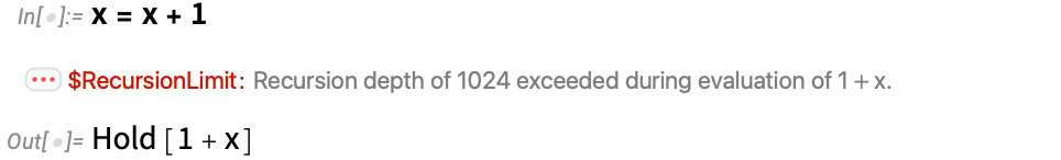
But over the years there’d been increasing evidence that this wasn’t quite adequate, and that for example further processing of the held form (even, for example, formatting it) could in extreme cases end up triggering even infinite cascades of evaluations. So finally—in Version 13.2 at the end of last year—we introduced the beginnings of a new mechanism to cut off “runaway” computations, based on a construct called TerminatedEvaluation:
\n
And from the beginning we wanted to see how to encode within TerminatedEvaluation information about just what evaluation had been terminated. But to do this once again seemed to require having a way to represent the “ongoing process of evaluation”—leading us back to Trace, and making us think about evaluation graphs, causal graphs, etc.
\nAt the beginning x = x + 1 might just have seemed like an irrelevant corner case—and for practical purposes it basically is. But already four decades ago it led me to start thinking not just about the results of computations, but also how their internal processes can be systematically organized. For years, I didn’t really connect this to my work on explicit computational processes like those in systems such as cellular automata. Hints of such connections did start to emerge as I began to try to build computational models of fundamental physics. But looking back I realize that in x = x + 1 there was already in a sense a shadow of what was to come in our Physics Project and in the whole construction of the ruliad.
\nBecause x = x + 1 is something which—like physics and like the ruliad—necessarily generates an ongoing process of computation. One might have thought that the fact that it doesn’t just “give an answer” was in a sense a sign of uselessness. But what we’ve now realized is that our whole existence and experience is based precisely on “living inside a computational process” (which, fortunately for us, hasn’t just “ended with an answer”). Expression evaluation is in its origins intended as a “human-accessible” form of computation. But what we’re now seeing is that its essence also inevitably encompasses computations that are at the core of fundamental physics. And by seeing the correspondence between what might at first appear to be utterly unrelated intellectual directions, we can expect to inform both of them. Which is what I have started to try to do here.
\nWhat I’ve described here builds quite directly on some of my recent work, particularly as covered in my books Combinators: A Centennial View and Metamathematics: Physicalization & Foundations. But as I mentioned above, I started thinking about related issues at the beginning of the 1980s in connection with the design of SMP, and I’d like to thank members of the SMP development team for discussions at that time, particularly Chris Cole, Jeff Greif and Tim Shaw. Thanks also to Bruce Smith for his 1990 work on Trace in Wolfram Language, and for encouraging me to think about symbolic representations of computational processes. In much more recent times, I’d particularly like to thank Jonathan Gorard for his extensive conceptual and practical work on multiway systems and their formalism, both in our Physics Project and beyond. Some of the directions described here have (at least indirectly) been discussed in a number of recent Wolfram Language design review livestreams, with particular participation by Ian Ford, Nik Murzin, and Christopher Wolfram, as well as Dan Lichtblau and Itai Seggev. Thanks also to Wolfram Institute fellows Richard Assar and especially Nik Murzin for their help with this piece.
\n", "category": "Computational Science", "link": "https://writings.stephenwolfram.com/2023/09/expression-evaluation-and-fundamental-physics/", "creator": "Stephen Wolfram", "pubDate": "Fri, 29 Sep 2023 21:48:31 +0000", "enclosure": "", "enclosureType": "", "image": "", "id": "", "language": "en", "folder": "", "feed": "wolfram", "read": false, "favorite": false, "created": false, "tags": [], "hash": "7936f5db0afca7e042169bdf56dcba3d", "highlights": [] }, { "title": "Remembering Doug Lenat (1950–2023) and His Quest to Capture the World with Logic", "description": "In many ways the great quest of Doug Lenat’s life was an attempt to follow on directly from the work of Aristotle and Leibniz. For what Doug was fundamentally trying to do over the forty years he spent developing his CYC system was to use the framework of logic—in more or less the same form that Aristotle and Leibniz had it—to capture what happens in the world. It was a noble effort and an impressive example of long-term intellectual tenacity. And while I never managed to actually use CYC myself, I consider it a magnificent experiment—that if nothing else ultimately served to demonstrate the importance of building frameworks beyond logic alone in usefully representing and reasoning about the world.
\nDoug Lenat started working on artificial intelligence at a time when nobody really knew what might be possible—or even easy—to do. Was AI (whatever that might mean) just a clever algorithm—or a new type of computer—away? Or was it all just an “engineering problem” that simply required pulling together a bigger and better “expert system”? There was all sorts of mystery—and quite a lot of hocus pocus—around AI. Did the demo one was seeing actually prove something, or was it really just a trivial (if perhaps unwitting) cheat?
\nI first met Doug Lenat at the beginning of the 1980s. I had just developed my SMP (“Symbolic Manipulation Program”) system, that was the forerunner of Mathematica and the modern Wolfram Language. And I had been quite exposed to commercial efforts to “do AI” (and indeed our VCs had even pushed my first company to take on the dubious name “Inference Corporation”, complete with a “=>” logo). And I have to say that when I first met Doug I was quite dismissive. He told me he had a program (that he called “AM” for “Automated Mathematician”, and that had been the subject of his Stanford CS PhD thesis) that could discover—and in fact had discovered—nontrivial mathematical theorems.
\n“What theorems?” I asked. “What did you put in? What did you get out?” I suppose to many people the concept of searching for theorems would have seemed like something remarkable, and immediately exciting. But not only had I myself just built a system for systematically representing mathematics in computational form, I had also been enumerating large collections of simple programs like cellular automata. I poked at what Doug said he’d done, and came away unconvinced. Right around the same time I happened to be visiting a leading university AI group, who told me they had a system for translating stories from Spanish into English. “Can I try it?” I asked, suspending for a moment my feeling that this sounded like science fiction. “I don’t really know Spanish”, I said, “Can I start with just a few words?” “No”, they said, “the system works only with stories.” “How long does a story have to be?” I asked. “Actually it has to be a particular kind of story”, they said. “What kind?” I asked. There were a few more iterations, but eventually it came out: the “system” translated one particular story from Spanish into English! I’m not sure if my response included an expletive, but I wondered what kind of science, technology, or anything else this was supposed to be. And when Doug told me about his “Automated Mathematician”, this was the kind of thing I was afraid I was going to find.
\nYears later, I might say, I think there’s something AM could have been trying to do that’s valid, and interesting, if not obviously possible. Given a particular axiom system it’s easy to mechanically generate infinite collections of “true theorems”—that in effect fill metamathematical space. But now the question is: which of these theorems will human mathematicians find “interesting”? It’s not clear how much of the answer has to do with the “social history of mathematics”, and how much is more about “abstract principles”. I’ve been studying this quite a bit in recent years (not least because I think it could be useful in practice)—and have some rather deep conclusions about its relation to the nature of mathematics. But I now do wonder to what extent Doug’s work from all those years ago might (or might not) contain heuristics that would be worth trying to pursue even now.
\nI ran into Doug quite a few times in the early to mid-1980s, both around a company called Thinking Machines (to which I was a consultant) and at various events that somehow touched on AI. There was a fairly small and somewhat fragmented AI community in those days, with the academic part in the US concentrated around MIT, Stanford and CMU. I had the impression that Doug was never quite at the center of that community, but was somehow nevertheless a “notable member”, who—particularly with his work being connected to math—was seen as “doing upscale things” around AI.
\nIn 1984 I wrote an article for a special issue of Scientific American on “computer software” (yes, software was trendy then). My article was entitled “Computer Software in Science and Mathematics”, and the very next article was by Doug, entitled “Computer Software for Intelligent Systems”. The summary at the top of my article read: “Computation offers a new means of describing and investigating scientific and mathematical systems. Simulation by computer may be the only way to predict how certain complicated systems evolve.” And the summary for Doug’s article read: “The key to intelligent problem solving lies in reducing the random search for solutions. To do so intelligent computer programs must tap the same underlying ‘sources of power’ as human beings”. And I suppose in many ways both of us spent most of our next four decades essentially trying to fill out the promise of these summaries.
\nA key point in Doug’s article—with which I wholeheartedly agree—is that to create something one can usefully identify as “AI”, it’s essential to somehow have lots of knowledge of the world built in. But how should that be done? How should the knowledge be encoded? And how should it be used?
\nDoug’s article in Scientific American illustrated his basic idea:
\n
Encode knowledge about the world in the form of statements of logic. Then find ways to piece together these statements to derive conclusions. It was, in a sense, a very classic approach to formalizing the world—and one that would at least in concept be familiar to Aristotle and Leibniz. Of course it was now using computers—both as a way to store the logical statements, and as a way to find inferences from them.
\nAt first, I think Doug felt the main problem was how to “search for correct inferences”. Given a whole collection of logical statements, he was asking how these could be knitted together to answer some particular question. In essence it was just like mathematical theorem proving: how could one knit together axioms to make a proof of a particular theorem? And especially with the computers and algorithms of the time, this seemed like a daunting problem in almost any realistic case.
\nBut then how did humans ever manage to do it? What Doug imagined was that the critical element was heuristics: strategies for guessing how one might “jump ahead” and not have to do the kind of painstaking searches that systematic methods seemed to imply would be needed. Doug developed a system he called EURISKO that implemented a range of heuristics—that Doug expected could be used not only for math, but basically for anything, or at least anything where human-like thinking was effective. And, yes, EURISKO included not only heuristics, but also at least some kinds of heuristics for making new heuristics, etc.
\nBut OK, so Doug imagined that EURISKO could be used to “reason about” anything. So if it had the kind of knowledge humans do, then—Doug believed—it should be able to reason just like humans. In other words, it should be able to deliver some kind of “genuine artificial intelligence” capable of matching human thinking.
\nThere were all sorts of specific domains of knowledge to consider. But Doug particularly wanted to push in what seemed like the most broadly impactful direction—and tackle the problem of commonsense knowledge and commonsense reasoning. And so it was that Doug began what would become a lifelong project to encode as much knowledge as possible in the form of statements of logic.
\nIn 1984 Doug’s project—now named CYC—became a flagship part of MCC (Microelectronics and Computer Technology Corporation) in Austin, TX—an industry-government consortium that had just been created to counter the perceived threat from the Japanese “Fifth Generation Computer Project”, that had shocked the US research establishment by putting immense resources into “solving AI” (and was actually emphasizing many of the same underlying rule-based techniques as Doug). And at MCC Doug had the resources to hire scores of people to embark on what was expected to be a few thousand person-years of effort.
\nI didn’t hear much about CYC for quite a while, though shortly after Mathematica was released in 1988 Marvin Minsky mused to me about how it seemed like we were doing for math-like knowledge what CYC was hoping to do for commonsense knowledge. I think Marvin wasn’t convinced that Doug had the technical parts of CYC right (and, yes, they weren’t using Marvin’s theories as much as they might). But in those years Marvin seemed to feel that CYC was one of the few AI projects going on that actually made any sense. And indeed in my archives I find a rather charming email from Marvin in 1992, attaching a draft of a science fiction novel (entitled The Turing Option) that he was writing with Harry Harrison, which contained mention of CYC:
\n\n\nJune 19, 2024
\n\nWhen Brian and Ben reached the lab, the computer was running
\nbut the tree-robot was folded and motionless. “Robin,
\nactivate.”
\n\n…
\n\n“Robin will have to use different concepts of progress for
\ndifferent kinds of problems. And different kinds of subgoals
\nfor reducing those different kinds of differences.”
\n\n“Won’t that require enormous amounts of knowledge?”
\n\n“It will indeed—and that’s one reason human education takes
\nso long. But Robin should already contain a massive amount of
\njust that kind of information—as part of his CYC-9 knowledge-
\nbase.”
\n\n…
\n\n“There now exists a procedural model for the behavior of a
\nhuman individual, based on the prototype human described in
\nsection 6.001 of the CYC-9 knowledge base. Now customizing
\nparameters on the basis of the example person Brian Delaney
\ndescribed in the employment, health, and security records of
\nMegalobe Corporation.”
\n\nA brief silence ensued. Then the voice continued.
\n\n“The Delaney model is judged as incomplete as compared to those
\nof other persons such as President Abraham Lincoln, who has
\n3596.6 megabytes of descriptive text, or Commander James
\nBond, who has 16.9 megabytes.”
Later, one of the novel’s characters observes: “Even if we started with nothing but the
\nold Lenat–Haase representation-languages, we’d still be far ahead of what any animal ever evolved.” (Ken Haase was a student of Marvin’s who critiqued and extended Doug’s work on heuristics.)
I was exposed to CYC again in 1996 in connection with a book called HAL’s Legacy—to which both Doug and I contributed—published in honor of the fictional birthday of the AI in the movie 2001. But mostly AI as a whole was in the doldrums, and almost nobody seemed to be taking it seriously. Sometimes I would hear murmurs about CYC, mostly from government and military contacts. Among academics, Doug would occasionally come up, but rather cruelly he was most notable for his name being used for a unit of “bogosity”—the lenat—of which it was said that “Like the farad it is considered far too large a unit for practical use, so bogosity is usually expressed in microlenats”.
\nMany years passed. I certainly hadn’t forgotten Doug, or CYC. And a few times people suggested connecting CYC in some way to our technology. But nothing ever happened. Then in the spring of 2009 we were nearing the first release of Wolfram|Alpha, and it seemed like I finally had something that I might meaningfully be able to talk to Doug about.
\nI sent a rather tentative email:
\n
I just made a small blog post about it:
\nhttp://blog.wolfram.com/2009/03/05/wolframalpha-is-coming/\n
\nI’d be pleased to give you a webconference demo if you’re interested.
\nI hope you’ve been well all these years.
\n— Stephen